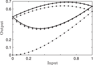
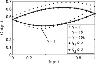
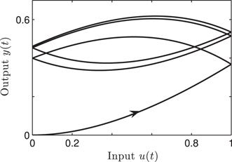
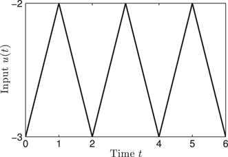
A Survey of the Hysteretic Duhem Model

  1. 1.Department of Mathematics, Barcelona East School of EngineeringUniversitat Politècnica de CatalunyaBarcelonaSpain
Original Paper

DOI: 10.1007/s11831-017-9218-3

Cite this article as:
Ikhouane, F. Arch Computat Methods Eng (2017). doi:10.1007/s11831-017-9218-3
  • 6 Downloads

Abstract

The Duhem model is a simulacrum of a complex and hazy reality: hysteresis. Introduced by Pierre Duhem to provide a mathematical representation of thermodynamical irreversibility, it is used to describe hysteresis in other areas of science and engineering. Our aim is to survey the relationship between the Duhem model as a mathematical representation, and hysteresis as the object of that representation.

1 Prolegomenon

Citing a reference allows the author of a scientific article to attribute work and ideas to the correct source. Nonetheless, the process of describing that work and these ideas assumes some interpretation, at least of their relative importance. In order to ensure that the interpretation is reliable, we use, whenever adequate, a quotation from the reference so that the reader has a direct access to the cited source. This direct access is even more important when the source is not easily available like Ref. [67]1 or is not written in English like Refs. [16, 17, 18, 19, 20, 21, 22] among others, in which case we provide a translation. This is our approach to the literature review of Sect. 2.

In Sects. 49 we proceed differently since our aim in these sections is to provide an accurate description of the results presented in the references under study. Because of the diversity of notations and nomenclature in these references, quotations may not be the best way to transmit that accurate description. Instead, we summarize the references using a unifying framework provided in Ref. [35]. The references we have chosen in Sects. 49 are, in our opinion, those that are relevant to the subject of this study.

Our aim in this work is also to shed light on the relationships between the concepts introduced in this paper. To this end, we use a special form of the Duhem model, the scalar semilinear one, as a case study.

2 Introduction and Literature Review

A brief history of the Duhem model The term hysteresis was coined by J. A. Ewing in 1881 to describe a specific relationship between the torsion of a magnetized wire and its polarization (although the phenomenon of hysteresis has been known and described by several authors before that date as shown in the literature review provided in Ref. [65]).

Quoting from Ewing’s paper [28]: “These curves exhibit, in a striking manner, a persistence of previous state, such as might be caused by molecular friction. The curves for the back and forth twists are irreversible, and include a wide area between them. The change of polarization lags behind the change of torsion. To this action the author now gives the name Hysterēsis ( to be behind)”.

In 1887 Lord Rayleigh models the relationship between a magnetizing force F[Fmax,Fmax]F[Fmax,Fmax] and the corresponding magnetization M using two polynomials [59, p. 240]:
M=αF+βF2max(112(1FFmax)2)
when F is decreasing,
M=αF+βF2max(1+12(1+FFmax)2)
when F is increasing, where α,α,ββ and FmaxFmax are constants.

However, the first in-depth study of hysteresis is due to Pierre Duhem2 in the period 1896–1902. A detailed review of Duhem’s work on hysteresis may be found in [67, Chapter IV] so that we provide here only those elements of that extensive work that are directly related to the present paper.

To understand the motivation for Duhem’s work we quote from [67, p. 306]: “take a metallic wire under strain by means of a load. We can take the length of the wire and its temperature as variables that define its state. The gravity weight P will represent the external action. At temperature T and under the load P the wire may be at equilibrium with length l. Give P infinitely small variations, the length l and temperature T will also experience infinitely small variations, and a new equilibrium may be achieved. In this last state, give the gravity weight and temperature variations equal in absolute value, but of opposite signs to the previous ones. The length l should experience a variation equal to the previous one with opposite sign. However, experimentation shows that this is not the case. In general, to the expansion of the wire corresponds a smaller contraction, and the difference lasts with time.”

This permanent deformation is the subject of a seven-memoirs research by Duhem, see Refs. [16]–[22]. In his first memoir submitted to the section of sciences of the Académie de Belgique on October 13, 1894, and reviewed by the mathematician Charles Lagrange in Ref. [44],3 Duhem writes: “The attempts to make the different kinds of permanent deformations compatible with the principles of thermodynamics have been few up till now. Only one of these attempts, due to M. Marcel Brillouin, appears to us worthy of interest.” [16, p. 3]. Duhem analyzes the work of Brillouin and concludes that it is not compatible with the principles of thermodynamics [16, p. 6] (see also [19, pp. 5–7]).

As an alternative, Duhem starts a theory of permanent deformations by considering the simplest case: that of a system defined by one normal variable x and its absolute temperature T. Denoting F(x,T)F(x,T) the internal thermodynamic potential of the system, Duhem writes [16, p. 8]: “Let X be the external action to which this system is subject. The condition of equilibrium of the system will be
X=F(x,T)x.
X=F(x,T)x.
(1)
Let (xTX) and (x+dx,T+dT,X+dX)(x+dx,T+dT,X+dX)be two equilibria of the system, infinitely close to each other; owing to equality [(1)] we get
dX=2F(x,T)x2dx+2F(x,T)xTdT.''
(2)
Equation (2) does not take into account the fact that the modifications of equilibria are not reversible. So Duhem introduces a term f(xTX)|dx| to be added to the right-hand side of Eq. (2), where f is a continuous function of the three variables x, T, and X. For an isothermal modification (that is when T is maintained constant) we get [16, pp. 9–10]:
dXdx={f1(x,T,X) for an increasing x,f2(x,T,X) for a decreasing x,
dXdx={f1(x,T,X)f2(x,T,X) for an increasing x, for a decreasing x,
(3)
where
f1(x,T,X)=2F(x,T)x2+f(x,T,X),f2(x,T,X)=2F(x,T)x2f(x,T,X).
f1(x,T,X)=f2(x,T,X)=2F(x,T)x2+f(x,T,X),2F(x,T)x2f(x,T,X).
(4)
Observe that, when the input is piecewise monotone, the model (3) is equivalent to the model (5) proposed in Refs. [3] and [43, p. 282]:
˙x(t)={ϕ(x(t),u(t))˙u(t) for ˙u(t)0,ϕr(x(t),u(t))˙u(t) for ˙u(t)0,
x˙(t)={ϕ(x(t),u(t))u˙(t)ϕr(x(t),u(t))u˙(t) for u˙(t)0, for u˙(t)0,
(5)
where ϕϕ and ϕrϕr are functions that satisfy some conditions, the function u is the input (which is x using Duhem’s notation), the function x the state (which is X using Duhem’s notation), and t is time.

To the best of our knowledge, the first reference that called the form (5) “Duhem model” is Ref. [48] in 1993.4 Indeed, the authors of Ref. [43] attributed erroneously Duhem’s model to Madelung [63, p. 797].5

Between 1916 when P. Duhem dies and 1993 when his model of hysteresis is finally attributed to him, Duhem’s work on hysteresis does not have a relevant impact. Major references on hysteresis like Refs. [8, 12] or [56] do not cite his memoirs. Several authors propose different forms of the Duhem model without a direct reference to Duhem’s memoirs. This is the case of the Coleman and Hodgdon model of magnetic hysteresis [12], the Dahl model of friction [13], the model (5) in Ref. [3], and a generalized form of the model (5) in Ref. [43, p. 95]. In 1952, Everett cites briefly Duhem’s work as follows [24, p. 751]: “From a thermodynamic standpoint the introduction of an additional variable whose value depends on the history of the system is sufficient for a formal discussion (cf. Duhem [ref][ref]). To advance our understanding of the phenomenon [of hysteresis], however, a molecular interpretation is desirable.”

A general theory of physics based on a molecular interpretation was precisely what Duhem rejected. In a review of his work presented in 1913 for his application to the Académie des Sciences, Duhem writes that his “doctrine should note imitate the numerous mechanical theories proposed by physicists hitherto; to the observable properties that apparatus measure, it will not substitute hidden movements of hypothetical bodies” [67, p. 74].

In recent times, Duhem’s phenomenological approach is becoming more accepted [5, 9, 46, 52, 57]. Indeed, “hysteretic phenomena arising in structural and mechanical systems are so complicated that there has been no well-accepted mathematical model which can describe all observed hysteretic characteristics.” [52, p. 1408]. Moreover, the Preisach model which was believed to describe the constitutive behavior of magnetic hysteresis, has shown to be a phenomenological model [49, p. 2].

Several reasons are invoked for the use of Duhem’s model to describe hysteresis. On the one hand, “differential equation-based models lead to a particularly simple phenomenological description” [46, p. C8–545]. On the other hand, the “Duhem models [sic] have the advantage that [they] require a small amount of memory so they are suitable in practical and low cost applications.” [9, p. 628]. Finally, many phenomenological models of friction or hysteresis can be seen as particular cases of a more general form of the Duhem model: this is the case for example of the Dahl [13], the LuGre [2, 11], or the Maxwell-slip models [30]. Thus “recast[ing] each model in the form of a generalized Duhem model provide[s] a unified framework for comparing the hysteretic nature of these models.”s [57, p. 91].

There are several generalizations of the original Duhem model (5). The following generalization is proposed in [43, p. 95]: ˙x(t)=f(t,x(t),u(t),˙u(t))x˙(t)=f(t,x(t),u(t),u˙(t)). In [64, p. 141] the terms ϕ(x(t),u(t))ϕ(x(t),u(t)) and ϕr(x(t),u(t))ϕr(x(t),u(t)) in (5) are replaced by [ϕ(x,u)](t)[ϕ(x,u)](t) and [ϕr(x,u)](t)[ϕr(x,u)](t) respectively, where ϕϕ and ϕrϕr are causal operators. In Ref. [54] Duhem’s model is generalized as ˙x(t)=f(x(t),u(t))g(˙u(t))x˙(t)=f(x(t),u(t))g(u˙(t)) whilst [64, p. 145] proposes the following form for vector hysteresis: ˙x(t)=f(x(t),u(t),π(˙u))|˙u(t)|x˙(t)=f(x(t),u(t),π(u˙))|u˙(t)| where π(˙u0)=˙u/|˙u|π(u˙0)=u˙/|u˙|.

Why are there different generalized forms of the Duhem model ? To answer this question we have to recall the concept of rate independence.6

To the best of our knowledge, the earliest author to state clearly rate independence is R. Bouc in Ref. [8], although that property was known before Bouc’s work. Due to the importance of rate independence in the study of hysteresis, and the fact that Ref. [8] is not available in English, we quote from [8, p. 17]:“Consider the graph with hysteresis of Fig. 1 where FFis not a function of x. To the valuex=x0x=x0correspond four values ofFF.
Fig. 1

Graph “Force–displacement” with hysteresis

If we consider now x as a function of time, the value of the force at instant t will depend not only on the value x(t), but also on all past values of function x since the origin instant where it is defined. If ββ is that instant (x(β)=F(β)=0,βx(β)=F(β)=0,β), then we denote F(t)=A(x(),t)F(t)=A(x(),t) the value of the force at instant “tt”, where x()x() “represents” the whole function on the interval [β,t][footnote][β,t][footnote]. Our aim is to explicit functional A(x(),t)A(x(),t).

To this end, we make the following assumption: the graph of Fig. 1 remains the same for all increasing function x()x() between 0 and x1x1, decreasing between the values x1x1 and x2x2, etc. The functional will no longer depend explicitly on time and we will write F(t)=A(x())(t)F(t)=A(x())(t). We can say: If x(tj)x(tj) and x(tj+1)x(tj+1) are two extremal values, consecutive in time, we have for all t[tj,tj+1]t[tj,tj+1]
A(x())(t)=fj(x(t)),
A(x())(t)=fj(x(t)),
where fjfj is a function of only the variable x(t).
We can also say: If ϕ:RRϕ:RR is a class C1C1 function whose derivative is strictly positive for tβtβ with ϕ(β)=βϕ(β)=β, and if we consider the function y(t)=x(ϕ(t))y(t)=x(ϕ(t)) which is a “compression” or an “expansion” of x by intervals, then the graphs (A(y()),y)(A(y()),y) and (A(x()),x)(A(x()),x) are identical and we have
A(x())(t)=A(y())(ϕ1(t)).''
The exact definition of rate independence varies from author to author. For example, Visintin requires the time-scale-change ϕϕ to be a strictly increasing time homeomorphism [64, p. 13] whilst Oh and Bernstein consider that ϕϕ is continuous, piecewise C1C1, nondecreasing, ϕ(0)=0ϕ(0)=0, and limtϕ(t)=limtϕ(t)= [54]. Loosely speaking, rate independence means that the graph of hysteresis (output versus input) is invariant with respect to any change in time scale.

Rate independence is used by Visintin to define hysteresis :“Definition. Hysteresis = Rate Independent Memory Effect.”[64, p. 13]. However, “this definition excludes any viscous-type memory” [64, p. 13] because it leads to rate-dependent effects that increase with velocity. A definition based on rate independence assumes that “the presence of hysteresis loops is not … an essential feature of hysteresis.” [64, p. 14].

This point of view is challenged by Oh and Bernstein who consider hysteresis as a “nontrivial quasi-dc input-output closed curve” [54, p. 631] and propose a modified version of the Duhem model which can represent rate-dependent or rate-independent effects. A characterization of hysteresis systems using hysteresis loops is also addressed by Ikhouane in Ref. [35] through the concepts of consistency and strong consistency.

In light of what has been said it becomes clear that, in Ref. [64], the generalizations of Duhem’s model are done in such a way that rate independence is preserved, whilst a definition of hysteresis based on hysteresis loops in Ref. [54] is compatible with a generalized form of the Duhem model that may be rate dependent or rate independent.

Why are there different models of hysteresis? In Ref. [16] Duhem proposes his model to account for the irreversibility in the modifications of equilibria observed experimentally in magnetic hysteresis [16, Chap. IV], sulfur [17], red phosphorus [19, Chap. III], and in different processes of metallurgy [19].

Preisach [56] uses “plausible hypotheses concerning the physical mechanisms of magnetization” [49, p. 1] to elaborate a model of magnetic hysteresis. This model is also proposed and studied by Everett and co-workers [24, 25, 26, 27] who postulate “that hysteresis is to be attributed in general to the existence in a system of a very large number of independent domains, at least some of which can exhibit metastability.” [24, p. 753].

Krasnosel’skiǐ and Pokrovskiǐ point out to the issue of admissible inputs, as “it is by no means clear a priori for any concrete transducer with hysteresis, how to choose the relevant classes of admissible inputs” [43, p. 5]. This is why they introduce the concept of vibro-correctness which allows the determination of the output of a hysteresis transducer that corresponds to any continuous input, once we know the outputs that correspond to piecewise monotone continuous inputs [43, p. 6]. The models that Krasnosel’skiǐ and Pokrovskiǐ propose (ordinary play, generalized play, hysteron) are vibro-correct, although the authors acknowledge the existence of hysteresis models that may not be vibro-correct like the Duhem model.7

Hysteresis models based on a feedback interconnection between a linear system and a static nonlinearity are proposed in Ref. [55]. The authors study “hysteresis arising from a continuum of equilibria … and hysteresis arising from isolated equilibria” [55, p 101].

A review of hysteresis models is provided in Ref. [48] and a detailed study of these (and other) models may be found in Refs. [7, 10, 14, 37], [49, 64].

In light of what has been said, the diversity of hysteresis models is due to the wide range of areas to which hysteresis is concomitant, and the diversity of methods and assumptions underlying the elaboration of these models.

Note that all mathematical models of hysteresis share a common property: they model hysteresis. This fact leads us to our next question.

What is hysteresis? A description found in many papers is that hysteresis “refers to the systems that have memory, where the effects of input to the system are experienced with a certain delay in time.” [33, p. 210]. This description is misleading as it applies also to dynamic linear systems. Indeed, when the output y is related to the input u by ˙x=Ax+Bux˙=Ax+Bu and y=Cxy=Cx which is a possible description of a linear system, the output is given by y(t)=C[exp(tA)x0+t0exp((tτ)A)Bu(τ)dτ]y(t)=C[exp(tA)x0+t0exp((tτ)A)Bu(τ)dτ] where x0x0 is the initial state and t0t0 is time. We can see that y(t) depends on the integral of a function that incorporates u(τ)u(τ) for all τ[0,t]τ[0,t], which means that the linear system does have memory. However, “hysteresis is a genuinely nonlinear phenomenon” [10, p. 7].

Mayergoyz considers hysteresis as a rate-independent phenomenon which is “consistent with existing experimental facts.” [49, p. 16]. However, “for very fast input variations, time effects become important and the given definition of rate-independent hysteresis fails.” [49, p. 16]. Also, “in the existing literature, hysteresis phenomenon is by and large linked with the formation of hysteresis loops (looping). This may be misleading and create the impression that looping is the essence of hysteresis. In this respect, the given definition of hysteresis emphasizes the fact that history dependent branching constitutes the essence of hysteresis, while looping is a particular case of branching.” [49, pp. 16–18].

Following Mayergoyz, “All rate-independent hysteresis nonlinearities fall into two general classifications: (a) hysteresis nonlinearities with local memories, and (b) hysteresis nonlinearities with nonlocal memories.” [49, pp. 17]. In a hysteresis with a local memory, the state or output at time tt0tt0 is completely defined by the state or output at instant t0t0, and the input on [t0,t][t0,t]. This is the case for example of a hysteresis given by a differential equation. Hysteresis with a nonlocal memory is a hysteresis which is not with local memory. This is the case for example of the Preisach model. “However, the notion of hysteresis nonlinearities with local memories is not consistent with experimental facts.” [49, pp. 19–20]. Hodgdon, on the other hand, writes in relation with the use of a special case of the Duhem model to represent ferromagnetic hysteresis: “These results are in good agreement with the manufacturer’s dc hysteresis data and with experiments” [34, p. 220].

In Ref. [54], Oh and Bernstein consider the generalized Duhem model ˙x=f(x,u)g(˙u)x˙=f(x,u)g(u˙) and y=h(x,u)y=h(x,u) with u the input, y the output and x the state. The authors assume the existence of a unique solution of the differential equation on the time interval [0,[[0,[. They also assume the existence of a T–periodic solution xTxT for any T–periodic input uTuT with one increasing part and one decreasing part, which means that the graph {(uT,xT)}{(uT,xT)} is a closed curve. Finally they assume that when TT the graph {(uT,xT)}{(uT,xT)} converges with respect to the Hausdorff metric to a closed curve CC. If we can find (a,b1)C(a,b1)C and (a,b2)C(a,b2)C with b1b2b1b2, the curve CC is not trivial and the generalized Duhem model is a hysteresis.

In a PhD thesis advised by Bernstein [15], Drinčić considers systems of the form ˙x=f(x,u)x˙=f(x,u) and y=h(x,u)y=h(x,u) for which hysteresis is defined as in Ref. [54]. The system is supposed to be step convergent, that is limtx(t)limtx(t) exists for all initial conditions and for all constant inputs. It is noted that there exists “a close relationship” [15, p. 6] between the curve CC and the input-output equilibria map, that is the set E={(u,h(limtx(t),u))}E={(u,h(limtx(t),u))} where u is constant and f(limtx(t),u)=0f(limtx(t),u)=0. In particular, the “system is hysteretic if the multivalued mapEEhas either a continuum of equilibria or a bifurcation” [15, p. 7].

In Ref. [6] Bernstein states that “a hysteretic system must be multistable; conversely, a multistable system is hysteretic if increasing and decreasing input signals cause the state to be attracted to different equilibria that give rise to different outputs.” Multistability means that “the system must have multiple attracting equilibria for a constant input value” [6].

In Ref. [50], Morris presents six examples of hysteresis systems taken from the areas of electronics, biology, mechanics, and magnetics; hysteresis being understood as a “characteristic looping behavior of the input-output graph” [50, p. 1]. The author explains the qualitative behavior of these systems from the point of view of multistability. For “the differential equations used to model the Schmitt trigger, cellular signaling and a beam in a magnetic field” it is observed that “these systems, all possess, for a range of constant inputs, several stable equilibrium points.” [50, p. 13]. The author observes that the systems are rate dependent for high input rates.

For the play operator, the Preisach model and the Bouc-Wen model which are rate independent, “these models present a continuum of equilibrium points.” [50, p. 13]. These observations lead the author to conclude that “hysteresis is a phenomenon displayed by forced dynamical systems that have several equilibrium points; along with a time scale for the dynamics that is considerably faster than the time scale on which inputs vary.” [50, p. 13]. Morris proposes the following definition.

“A hysteretic system is one which has (1) multiple stable equilibrium points and (2) dynamics that are considerably faster than the time scale at which inputs are varied.” [50, p. 13].

In Ref. [35], Ikhouane considers a hysteresis operator “HHthat associates to an input u and initial conditionξ0ξ0 an output y=H(u,ξ0)y=H(u,ξ0), all belonging to some appropriate spaces.” [35, p. 293]. It is assumed that the operator HH is causal and satisfies the property that constant inputs lead to constant outputs. Examples include all rate-independent models [47, Proposition 2.1], some rate-dependent models, models with local memory like the various generalizations of the Duhem model, and models with nonlocal memory like the Preisach model.

The author introduces two changes in time scale: (1) a linear one which is applied to a given input, and (2) a -possibly- nonlinear one which is the total variation of the original input. When the input is composed with the linear time-scale change, both the input and the output are re-scaled with respect to the total variation of the input, which provides a normalized input independent of the linear time-scale change, and a normalized output. Consistency is defined as being the convergence of the normalized outputs in the space LL endowed with the uniform convergence norm. It is shown that consistency implies the convergence to some set of the graphs output versus input of the hysteresis operator when the linear time scale varies [35, Lemma 9].

Strong consistency is defined as the property that the limit of the normalized outputs, seen a parametrized curve, converges to a periodic orbit which characterizes the hysteresis loop.

The author does not propose a definition of hysteresis, but considers that consistency and strong consistency are properties of a class of hysteresis systems.

Aim of the paper The aim of the paper is to survey the research carried out on the Duhem model from the perspective of its hysteretic properties.

Organization of the paper Section 4 presents some results obtained in Ref. [43], namely the concept of vibro-correctness, sufficient conditions to ensure global solutions of the scalar rate independent Duhem model, and a study of the continuity of the model seen as an operator. Section 5 presents a definition of hysteresis proposed in Ref. [54] that uses a generalized form of Duhem’s model as a tool to get that formal definition. Section 6 presents the concepts of consistency and strong consistency introduced in Ref. [35]. The tools and notations of Ref. [35] are also used as a unifying framework to present the results of the present paper. Section 7 presents a characterization of the generalized Duhem model obtained in Ref. [51]. Section 8 summarizes the results obtained in Ref. [40] in relation with the study of the dissipativity of the Duhem model. Section 9 summarizes some results obtained in Ref. [64] in relation with the existence of a Duhem operator, its smoothness, and some generalizations of the model. Section 10 is a note that explores the minor loops of hysteresis systems with particular emphasis on the Duhem model. For ease of reference, some results on the existence and uniqueness of the solutions of differential equations are presented in Appendix 15.

To illustrate the results obtained in Sects. 410, and to analyze the relationships between these results, we use the scalar semilinear Duhem model as a case study. The corresponding mathematical analysis is stated in various lemmas and theorems provided in Section 11, whose proofs are given in 1620. The relationships between the results obtained in Sects. 49 are commented upon in Section 12. These comments lead to the formulation of several open problems in Sect. 13 and a conjecture in Sect. 11.9.

3 Terminology and Notations

A real number x is said to be strictly positive when x>0x>0, strictly negative when x<0x<0, nonpositive when x0x0, and nonnegative when x0x0. A function h:RRh:RR is said to be strictly increasing when t1<t2h(t1)<h(t2)t1<t2h(t1)<h(t2), strictly decreasing when t1<t2h(t1)>h(t2)t1<t2h(t1)>h(t2), nonincreasing when t1<t2h(t1)h(t2)t1<t2h(t1)h(t2), and nondecreasing when t1<t2h(t1)h(t2)t1<t2h(t1)h(t2).8

An ordered pair ab is denoted (ab) whilst the open interval {tRa<t<b}{tRa<t<b} is denoted ]ab[. The set of nonnegative integers is denoted N={0,1,}N={0,1,} and the set of nonnegative real numbers is denoted R+=[0,[R+=[0,[.

The Lebesgue measure on RR is denoted μμ. We say that a subset of RR is measurable when it is Lebesgue measurable. Let IR+IR+ be an interval, and consider a function ϕ:IRlϕ:IRl where l>0l>0 is an integer. We say that ϕϕ is measurable when ϕϕ is (Mμ,B)(Mμ,B)–measurable where B is the class of Borel sets of RlRl and MμMμ is the class of measurable sets of R+R+ [66]. For a measurable function ϕ:IRlϕ:IRl, ϕIϕI denotes the essential supremum of the function |ϕ||ϕ| on I where |||| is the Euclidean norm on RlRl. When I=R+I=R+, this essential supremum is denoted ϕϕ.

W1,(R+,Rl)W1,(R+,Rl) denotes the Sobolev space of absolutely continuous functions ϕ:R+Rlϕ:R+Rl. For this class of functions, we have ϕ<ϕ<; the derivative of ϕϕ is denoted ˙ϕϕ˙; this derivative is defined almost everywhere and satisfies ˙ϕ<ϕ˙<. Endowed with the norm ϕW1,(R+,Rl)=max(ϕ,˙ϕ)ϕW1,(R+,Rl)=max(ϕ,ϕ˙), the vector space W1,(R+,Rl)W1,(R+,Rl) is a Banach space [45, pp. 280–281].

L(R+,Rl)L(R+,Rl) denotes the Banach space of measurable and essentially bounded functions ϕ:R+Rlϕ:R+Rl endowed with the norm .

C0(R+,Rl)C0(R+,Rl) denotes the Banach space of continuous functions ϕ:R+Rlϕ:R+Rl endowed with the norm .

γ]0,[γ]0,[, the linear time-scale-change sγ:R+R+sγ:R+R+ is defined by the relation sγ(t)=t/γ,tR+sγ(t)=t/γ,tR+.

limxalimxa sets for limxax<alimxax<a whilst limxalimxa sets for limxax>alimxax>a.

Let U be a set and let T]0,[T]0,[. The function ϕ:R+Uϕ:R+U is said to be T–periodic if ϕ(t)=ϕ(t+T),tR+ϕ(t)=ϕ(t+T),tR+.

4 A Summary of the Results Obtained in Ref. [43]

This section presents those results obtained in Ref. [43] that are relevant to the present paper. This is in particular the case of the concept of vibro-correctness which allows to extend the set of admissible inputs from continuously differentiable to continuous.

4.1 The Concept of Vibro-Correctness

Consider the differential equation [43, p. 95]
˙x(t)=ζ1(t,x(t),u(t),˙u(t)),
x˙(t)=ζ1(t,x(t),u(t),u˙(t)),
(6)
x(t0)=x0.
x(t0)=x0.
(7)
In Eqs. (6)–(7) the initial time t0Rt0R and the initial state x0Rnx0Rn where n>0n>0 is an integer. Furthermore, the function ζ1:R×Rn×R×RRnζ1:R×Rn×R×RRn is continuous and the input uC1([t0,[,R)uC1([t0,[,R). Theorem 10 ensures the existence of at least a solution of (6)–(7) on some time interval [t0,t0[[t0,t0[ where t0>t0t0>t0 may be finite or infinite. Is it possible to extend the set of inputs from continuously differentiable to solely continuous? The answer to this question leads to the concept of vibro-correctness.
Let t1]t0,[t1]t0,[ and vC0([t0,t1],R)vC0([t0,t1],R). For any δ]0,[δ]0,[ define the set
E(δ,v)={uC1([t0,t1],R)uv[t0,t1]δ}.
(8)

Definition 1

[43, pp. 95–96] The differential equation (6)–(7) is vibro-correct if for each x0Rnx0Rn and each input uC0([t0,[,R)uC0([t0,[,R) there exist t1]t0,[t1]t0,[ and δ0]0,[δ0]0,[ such that Propreties (i)–(ii) hold.
  1. (i)

    uE(δ0,u)uE(δ0,u) the solution x=W(u,x0)x=W(u,x0) of Eqs. (6)–(7) exists and is unique on the time interval [t0,t1][t0,t1].

     
  2. (ii)

    limδsupu,vE(δ,u)W(u,x0)W(v,x0)[t0,t1]=0limδsupu,vE(δ,u)W(u,x0)W(v,x0)[t0,t1]=0.


In the following we analyze the consequences of vibro-correctness. Consider a sequence of inputs ukE(δ0,u)ukE(δ0,u) such that limkuku[t0,t1]=0limkuku[t0,t1]=0. Then, owing to Proprety (ii) of Definition 1, it follows that {W(uk,x0)}kN{W(uk,x0)}kN is a Cauchy sequence in C0([t0,t1],R)C0([t0,t1],R). Thus it converges with respect to the norm to a function xC0([t0,t1],R)xC0([t0,t1],R). Note that the function xx is independent of the particular choice of the sequence ukuk owing to Proprety (ii) of Definition 1. Defining W(u,x0)W(u,x0) as being xx means that the operator WW has been extended to the set of continuous inputs.

Thus, the concept of vibro-correctness allows to extend the definition of the operator WW from the set of continuously differentiable inputs to that of continuous inputs.

Another consequence of Property (ii) is the uniqueness of the solutions of (6)–(7). This means that it is not necessary to state explicitly in Property (i) that the differential equation (6)–(7) has a unique solution (this is what is done in Ref. [43]; see also [43, p. 104]).

Definition 2

[43, p. 98] If we consider only constant inputs uu in Definition 1 then the differential equation (6)–(7) is said to be vibro-correct on constant inputs.

Theorem 1

[43, p. 98] If the differential equation (6)–(7) is vibro-correct on constant inputs then we can find functionsζ2,ζ3:R×Rn×RRnζ2,ζ3:R×Rn×RRn such that for all(t,x,u,v)R×Rn×R×R(t,x,u,v)R×Rn×R×R we haveζ1(t,x,u,v)=ζ2(t,x,u)v+ζ3(t,x,u)ζ1(t,x,u,v)=ζ2(t,x,u)v+ζ3(t,x,u).

Theorem 1 means that the only differential equations (6)–(7) that may be vibro-correct are the ones that have the following form:
˙x(t)=ζ2(t,x(t),u(t))˙u(t)+ζ3(t,x(t),u(t)),
x˙(t)=ζ2(t,x(t),u(t))u˙(t)+ζ3(t,x(t),u(t)),
(9)
x(t0)=x0.
x(t0)=x0.
(10)

4.2 Global Solutions of the Scalar Rate-Independent Duhem Model

Consider the space S(t0,t2)S(t0,t2) of absolutely continuous functions u:[t0,t2]Ru:[t0,t2]R such that
uS=|u(t0)|+t2t0|˙u(t)|dt<,
uS=|u(t0)|+t2t0|u˙(t)|dt<,
(11)
where t2]t0,[t2]t0,[ is fixed. Consider following differential equation [43, p. 286]:
˙x(t)=h(x(t),u(t))˙u(t) for almost all t[t0,t2] such that ˙u(t)0,
x˙(t)=h(x(t),u(t))u˙(t) for almost all t[t0,t2] such that u˙(t)0,
(12)
˙x(t)=hr(x(t),u(t))˙u(t) for almost all t[t0,t2] such that ˙u(t)0,
x˙(t)=hr(x(t),u(t))u˙(t) for almost all t[t0,t2] such that u˙(t)0,
(13)
x(t0)=x0,
x(t0)=x0,
(14)
where uS(t0,t2)uS(t0,t2), and x(t)Rx(t)R. The functions h,hr:R×RRh,hr:R×RR are Borel, locally bounded,9 and satisfy the following unilateral Lipschitz conditions with respect to the first variable [43, p. 278]:
(x1x2)(h(x1,v)h(x2,v))λ(v)(x1x2)2,x1,x2R,v[au,bu],
(15)
(x1x2)(hr(x1,v)hr(x2,v))λ(v)(x1x2)2,x1,x2R,v[au,bu],
(16)
where λ:RR+λ:RR+ is continuous, au=mint[t0,t2]u(t)au=mint[t0,t2]u(t), and bu=maxt[t0,t2]u(t)bu=maxt[t0,t2]u(t). Observe that (15)–(16) are the transcription of (133) for the differential equation (12)–(13). Given that the function λλ is continuous, it is bounded on the interval [au,bu][au,bu] so that the term λ(v)λ(v) in Inequalities (15)–(16) can be replaced by a constant. Thus there exists a unique solution to (12)–(14) whose maximal interval of existence is [t0,t2][t0,t2] owing to Lemma 12.

4.3 Continuity of the Rate-Independent Duhem Model Seen as an Operator

For any given initial condition x0Rx0R define the operator Zx0:S(t0,t2)S(t0,t2)Zx0:S(t0,t2)S(t0,t2) that associates to each input uS(t0,t2)uS(t0,t2) the solution x of the differential equation (12)–(14). Then,

Theorem 2

[43, Theorem 29.1] The operatorZx0Zx0 is continuous. Furthermore, leta]0,[a]0,[, then

sup{uS(t0,t2)uSa}Zx0(u)S<sup{uS(t0,t2)uSa}Zx0(u)S<.

5 A Summary of the Results Obtained in Ref. [54]

This section presents those results obtained in Ref. [54] that are relevant to the present paper. In particular, the authors of Ref. [54] propose a definition that decides whether a given generalized Duhem model is a hysteresis or not.

5.1 The Generalized Duhem Model

The generalized Duhem model with input u, state x and output y consists of a differential equation that describes the state x as [54]
˙x(t)=f(x(t),u(t))g(˙u(t)), for almost all tR+,
x˙(t)=f(x(t),u(t))g(u˙(t)), for almost all tR+,
(17)
x(0)=x0,
x(0)=x0,
(18)
and an algebraic equation that describes the output y as
y(t)=h(x(t),u(t)),tR+.
(19)
In Eqs. (17)–(19) the input uW1,(R+,R)uW1,(R+,R);10 the function f:Rn×RRn×nf:Rn×RRn×n is continuous; n and nn are strictly positive integers; the function g:RRng:RRn is continuous and satisfies g(0)=0g(0)=0; the function h:Rn×RRh:Rn×RR is continuous; and the initial state x0Rnx0Rn. The following is assumed in [54, Section II, p. 633].

Assumption 1

For every (u,x0)W1,(R+,R)×Rn(u,x0)W1,(R+,R)×Rn there exists a unique solution xW1,(R+,Rn)xW1,(R+,Rn) that satisfies Eqs. (17)–(18).

From Assumption 1 we get yC0(R+,R)L(R+,R)yC0(R+,R)L(R+,R).

Define the operator Ho:W1,(R+,R)×RnC0(R+,R)L(R+,R)Ho:W1,(R+,R)×RnC0(R+,R)L(R+,R) by the relation Ho(u,x0)=yHo(u,x0)=y; and the operator Hs:W1,(R+,R)×RnW1,(R+,Rn)Hs:W1,(R+,R)×RnW1,(R+,Rn) by the relation Hs(u,x0)=xHs(u,x0)=x.

5.2 Definition of Hysteresis According to Ref. [54]

We stress that Ref. [54] does not propose a definition of hysteresis in general. Instead, the authors of Ref. [54] propose a definition that decides whether a given generalized Duhem model is a hysteresis or not (this is Definition 4). We now present the different steps that are followed in Ref. [54] to come to Definition 4.

Definition 3

The nonempty set CR2CR2 is a closed curve if there exists T]0,[T]0,[, a continuous, piecewise C1C1, and T–periodic function η:[0,T]R2η:[0,T]R2 such that η([0,T])=Cη([0,T])=C and η(0)=η(T)η(0)=η(T).

Note that Definition 3 is equivalent to [54, Definition 2.1]. Let umin,umaxRumin,umaxR with umin<umaxumin<umax and let α1,TRα1,TR with 0<α1<T0<α1<T. Consider a T–periodic input u:R+[umin,umax]u:R+[umin,umax] such that
  1. (i)

    the function u is continuous on R+R+,

     
  2. (ii)

    the function u is continuously differentiable on ]0,α1[]0,α1[ and on ]α1,T[]α1,T[ with ˙u<u˙<,

     
  3. (iii)

    the function u is strictly increasing on ]0,α1[]0,α1[ and is strictly decreasing on ]α1,T[]α1,T[,

     
  4. (iv)

    we have u(0)=u(T)=uminu(0)=u(T)=umin and u(α1)=umaxu(α1)=umax.

     
Let Λumin,umax,α1,TΛumin,umax,α1,T be the set of all such inputs u, and define the set
Λ=umin<umax0<α1<TΛumin,umax,α1,T.
(20)
Let γ]0,[γ]0,[; observe that the input usγusγ is TγTγ–periodic where sγsγ is a linear time-scale change. The following is assumed in [54, Definition 2.2].

Assumption 2

Under Assumption 1, for every uΛuΛ there exists a unique11 initial condition x0,uRnx0,uRn such that Hs(u,x0,u)Hs(u,x0,u) is also T–periodic.

In the following, to simplify the notations, the initial condition x0,usγx0,usγ for γ]0,[γ]0,[ is denoted simply x0,γx0,γ. Note that, owing to the continuity and periodicity of Hs(usγ,x0,γ)Hs(usγ,x0,γ), we have [Hs(usγ,x0,γ)](0)=[Hs(usγ,x0,γ)](Tγ)[Hs(usγ,x0,γ)](0)=[Hs(usγ,x0,γ)](Tγ). This fact, combined with Eq. (19) implies that the output Ho(usγ,x0,γ)Ho(usγ,x0,γ) is also TγTγ–periodic and that [Ho(usγ,x0,γ)](0)=[Ho(usγ,x0,γ)](0)=[Ho(usγ,x0,γ)](Tγ)[Ho(usγ,x0,γ)](Tγ). Define the closed curve
Cu,γ={(usγ(t),[Ho(usγ,x0,γ)](t)),t[0,Tγ]}.
(21)
Now, we introduce the so-called Hausdorff distance. Let k2k2 be an integer. For any two nonempty compact sets S1S1 and S2S2 in RkRk, define the Hausdorff distance dkdk by the relation
dk(S1,S2)=max{supη1S1(infη2S2|η1η2|),supη2S2(infη1S1|η1η2|)}.
(22)
Then, the collection of all nonempty compact subsets of RkRk is a complete metric space with respect to the Hausdorff distance dkdk [23, p. 67].

Definition 4

[54, Definition 2.2] Under Assumptions 1 and 2, the operator HoHo is a hysteresis if Conditions (i) and (ii) hold for all (u,x0)Λ×Rn(u,x0)Λ×Rn.
  1. (i)

    There exists a closed curve CuR2CuR2 such that limγd2(Cu,Cu,γ)=0limγd2(Cu,Cu,γ)=0.

     
  2. (ii)

    There exist a,b1,b2Ra,b1,b2R with b1b2b1b2 such that (a,b1)Cu(a,b1)Cu and (a,b2)Cu(a,b2)Cu.


Remark 1

Condition (i) in Definition 4 states that limγd2(Cu,Cu,γ)=0limγd2(Cu,Cu,γ)=0. For this reason, it is not necessary that γ]0,[γ]0,[ in Assumption 2, it suffices that γ0]0,[γ0]0,[ such that the condition in Assumption 2 holds for all γ]γ0,[γ]γ0,[.

Remark 2

Owing to Theorem 1, the generalized Duhem model (17)–(19) is not vibro-correct when the function g is not linear. This implies that it cannot be extended to continuous inputs by the use of the concept of vibro-correctness [43, p. 279]. If g is linear it is shown in [54, Proposition 3.2] that, for uΛuΛ, the state x can be written as a function of the input u which means that Condition (ii) of Definition 4 cannot be met.

5.3 Case Study

The semilinear Duhem model is used to illustrate Definition 4 and to analyze the relationship between Definition 4 and the concept of strong consistency presented in Sect. 6. To this end Section 11.5 provides an analytical study of the conditions under which the scalar semilinear Duhem model is a hysteresis according to Definition 4. This study is illustrated by numerical simulations in Sect. 11.6. Finally the relationship between Definition 4 and strong consistency is analyzed in Sect. 12.1.

6 A Summary of the Results Obtained in Ref. [35]

This section presents those results obtained in Ref. [35] that are relevant to the present paper. This is in particuler the case for the concepts of consistency and strong consistency.

6.1 The Normalized Input

Let p>0p>0 be an integer. For uW1,(R+,Rp)uW1,(R+,Rp), let ρu:R+R+ρu:R+R+ be the total variation of u on [0, t], that is ρu(t)=t0|˙u(τ)| d τR+ρu(t)=t0|u˙(τ)| d τR+, tR+tR+. The function ρuρu is well defined, nondecreasing and absolutely continuous. Observe that ρuρu may not be invertible (this happens when the input u is constant on some interval or intervals). Denote ρu,max=limtρu(t)ρu,max=limtρu(t) and let
  • Iu=[0,ρu,max]Iu=[0,ρu,max] if ρu,max=ρu(t)ρu,max=ρu(t) for some tR+tR+ (in this case the interval IuIu is finite),

  • Iu=[0,ρu,max[Iu=[0,ρu,max[ if ρu,max>ρu(t)ρu,max>ρu(t) for all tR+tR+ (in this case the interval IuIu may be finite or infinite).

Lemma 1

[35] LetuW1,(R+,Rp)uW1,(R+,Rp) be non constant12 so that the intervalIuIu is not reduced to a single point. Then there exists a unique functionψuW1,(Iu,Rp)ψuW1,(Iu,Rp) that satisfiesψuρu=uψuρu=u. Moreover, the functionψuψu satisfies˙ψuIu=1ψ˙uIu=1 and

μ({ϱIu˙ψu(ϱ) is  not  defined  or |˙ψu(ϱ)|1})=0μ({ϱIuψ˙u(ϱ) is  not  defined  or |ψ˙u(ϱ)|1})=0.

The function ψuψu is constructed as follows. Let ϱIuϱIu, then there exists tϱR+tϱR+ such that ρu(tϱ)=ϱρu(tϱ)=ϱ (note that tϱtϱ is not necessarily unique as ρuρu is not necessarily invertible). Then, u(tϱ)u(tϱ) is independent of the particular choice of tϱtϱ, and ψu(ϱ)ψu(ϱ) is defined by the relation ψu(ϱ)=u(tϱ)ψu(ϱ)=u(tϱ) [35].

Lemma 1 shows that the input u has been “normalized” so that the resulting function ψuψu is such that ˙ψuψ˙u has norm 1 with respect to the new time variable ϱϱ. For this reason, we call function ψuψu the normalized input.

For every γ]0,[γ]0,[ recall the linear time-scale-change sγsγ.

Lemma 2

[35] γ]0,[,Iusγ=Iuγ]0,[,Iusγ=Iu and ψusγ=ψuψusγ=ψu.

6.2 Class of Operators

Let Ξ,U,YΞ,U,Y be arbitrary sets. Let UU be the set of functions u:R+Uu:R+U, and YY the set of functions y:R+Yy:R+Y. Consider a function (called operator in this work) H:U×ΞYH:U×ΞY. The operator HH is said to be causal if the following holds [64, p. 60]: u1,u2U,x0Ξ,τ]0,[u1,u2U,x0Ξ,τ]0,[, if t[0,τ],u1(t)=u2(t)t[0,τ],u1(t)=u2(t), then t[0,τ],[H(u1,x0)](t)=[H(u2,x0)](t)t[0,τ],[H(u1,x0)](t)=[H(u2,x0)](t).

Assumption 3

[35] Let ΞΞ be a set of initial conditions. Consider a causal operator H:W1,(R+,Rp)×ΞL(R+,Rm)H:W1,(R+,Rp)×ΞL(R+,Rm) where mN{0}mN{0}. For every (u,x0,θ)W1,(R+,Rp)×Ξ×R+(u,x0,θ)W1,(R+,Rp)×Ξ×R+, if u is constant on the interval [θ,[[θ,[, then H(u,x0)H(u,x0) is constant on the same interval [θ,[[θ,[.

6.3 The Normalized Output

Lemma 3

[35] LetΞΞ be a set of initial conditions. Assume that the operatorH:W1,(R+,Rp)×ΞL(R+,Rm)H:W1,(R+,Rp)×ΞL(R+,Rm) is causal and satisfies Assumption3. Let (u,x0)W1,(R+,Rp)×Ξ(u,x0)W1,(R+,Rp)×Ξ. Then, there exists a unique functionφuL(Iu,Rm)φuL(Iu,Rm) that satisfiesφuρu=H(u,x0)φuρu=H(u,x0). Moreover, we haveφuIuH(u,x0)φuIuH(u,x0). IfH(u,x0)H(u,x0) is continuous onR+R+, thenφuφu is continuous onIuIu and we haveφuIu=H(u,x0)φuIu=H(u,x0).

The function φuφu, called normalized output, is constructed as follows. Let ϱIuϱIu, then there exists a not necessarily unique tϱR+tϱR+ such that ρu(tϱ)=ϱρu(tϱ)=ϱ. Then, [H(u,x0)](tϱ)[H(u,x0)](tϱ) is independent of the particular choice of tϱtϱ, and φu(ϱ)φu(ϱ) is defined by the relation φu(ϱ)=[H(u,x0)](tϱ)φu(ϱ)=[H(u,x0)](tϱ) [35].

Note that the correct notation for function φuφu is φu,x0,Hφu,x0,H to stress that this function depends also on the initial condition x0x0 and on the operator HH. However, in the definition of consistency (Definition 5), neither the initial condition x0x0 nor the operator HH vary, which justifies the simplified notation.

6.4 Definition of Consistency

The concept of consistency is introduced in Ref. [35] as follows.13 Consider that the input u is composed with the time-scale-change sγsγ where γ]0,[γ]0,[. Then, consider the set
Su,γ={(usγ(t),[H(usγ,x0)](t)),tR+}
(23)
which is the output H(usγ,x0)H(usγ,x0) versus the input usγusγ (observe that the initial condition x0x0 does not vary with γγ). Using the notations of Sects. 6.1 and 6.3 we get ψusγρusγ=usγψusγρusγ=usγ and φusγρusγ=H(usγ,x0)φusγρusγ=H(usγ,x0) for all γ]0,[γ]0,[. Thus, the set Su,γSu,γ can be rewritten as
Su,γ={(ψusγρusγ(t),φusγρusγ(t)),tR+},
(24)
which leads to
Su,γ={(ψusγ(ϱ),φusγ(ϱ)),ϱIusγ}.
(25)
Using Lemma 2 it follows from Eq. (25) that
Su,γ={(ψu(ϱ),φusγ(ϱ)),ϱIu}.
(26)
Observe that, in the expression (26) of the set Su,γSu,γ, the only term that depends on γγ is the function φusγL(Iu,Rm)φusγL(Iu,Rm).

Definition 5

[35] Let ΞΞ be a set of initial conditions. Consider a causal operator H:W1,(R+,Rp)×ΞL(R+,Rm)H:W1,(R+,Rp)×ΞL(R+,Rm) that satisfies Assumption 3. Let (u,x0)W1,(R+,Rp)×Ξ(u,x0)W1,(R+,Rp)×Ξ. The operator HH is said to be consistent with respect to(u,x0)(u,x0) if there exists a function φuL(Iu,Rm)φuL(Iu,Rm) such that limγφusγφuIu=0.limγφusγφuIu=0.

Define the set SuSu by the relation
Su={(ψu(ϱ),φu(ϱ)),ϱIu}.
(27)
Recall that the Hausdorff distance dp+mdp+m is defined by Eq. (22).

Lemma 4

[35] LetΞΞ be a set of initial conditions. Assume that the operatorH:W1,(R+,Rp)×ΞL(R+,Rm)H:W1,(R+,Rp)×ΞL(R+,Rm) is causal and satisfies Assumption3. If HH is consistent with respect to(u,x0)(u,x0) thenlimγdp+m(ˉSu,γ,ˉSu)=0limγdp+m(S¯u,γ,S¯u)=0, where ˉXX¯ is the closure of the set X.

The converse of Lemma 4 is not true in general [35, Example 2].

Definition 6

14 Let ΞΞ be a set of initial conditions. Consider a causal operator H:W1,(R+,Rp)×ΞL(R+,Rm)H:W1,(R+,Rp)×ΞL(R+,Rm) that satisfies Assumption 3. We say that HH is rate independent with respect to linear time-scale changes if (u,x0,γ)W1,(R+,Rp)×Ξ×]0,[(u,x0,γ)W1,(R+,Rp)×Ξ×]0,[ we have H(usγ,x0)=H(u,x0)sγH(usγ,x0)=H(u,x0)sγ almost everywhere.

Assumption 4

Let ΞΞ be a set of initial conditions. Consider a causal operator H:W1,(R+,Rp)×ΞL(R+,Rm)C0(R+,Rm)H:W1,(R+,Rp)×ΞL(R+,Rm)C0(R+,Rm) that satisfies Assumption 3. Assume that HH is consistent with respect to all (u,x0)W1,(R+,Rp)×Ξ(u,x0)W1,(R+,Rp)×Ξ.

The new element that Assumption 4 introduces is that the output H(u,x0)H(u,x0) is assumed to be continuous.

Proposition 1

Under Assumption 4, let the operator H:W1,(R+,Rp)×ΞL(R+,Rm)C0(R+,Rm)H:W1,(R+,Rp)×ΞL(R+,Rm)C0(R+,Rm) be defined by the relation H(u,x0)=φuρuH(u,x0)=φuρu. Then HH is causal, satisfies Assumption 3, and is rate independent with respect to linear time-scale changes.

Proof

Straightforward.

Under Assumption 4 write the operator HH as
H=H+H,
H=H+H,
(28)
H=HH.
H=HH.
(29)
For any (u,x0,γ)W1,(R+,Rp)×Ξ×]0,[(u,x0,γ)W1,(R+,Rp)×Ξ×]0,[ we have H(usγ,x0)=H(usγ,x0)H(u,x0)sγH(usγ,x0)=H(usγ,x0)H(u,x0)sγ. On the other hand, H(usγ,x0)=φusγρusγH(usγ,x0)=φusγρusγ and H(u,x0)sγ=φuρusγH(u,x0)sγ=φuρusγ. By Lemma 3 it follows that H(usγ,x0)=φusγφuIuH(usγ,x0)=φusγφuIu. Since the operator HH is consistent by Assumption 4 it follows that limγφusγφuIu=0limγφusγφuIu=0. We thus conclude that
limγH(usγ,x0)=0.
limγH(usγ,x0)=0.
(30)
The interpretation of Eqs. (28)–(30) is postponed to Section 12.1.3.

6.5 Definition of Strong Consistency

Observe that, in Definition 5 of consistency, the input u may be periodic or not. However, to characterize the hysteresis loop of the operator HH, the input u needs to be periodic. For this reason, Ref. [35] introduces the concept of strong consistency (this is Definition 7) in relation with periodic inputs.15

Lemma 5

[35] LetT]0,[T]0,[. IfuW1,(R+,Rp)uW1,(R+,Rp) is non constant andTperiodic, thenIu=R+Iu=R+ andψuW1,(R+,Rp)ψuW1,(R+,Rp) is ρu(T)ρu(T)periodic.

Definition 7

[35] Let ΞΞ be a set of initial conditions and let x0Ξx0Ξ. Let uW1,(R+,Rp)uW1,(R+,Rp) be such that the input u is non constant and T–periodic where T]0,[T]0,[. Consider an operator H:W1,(R+,Rp)×ΞL(R+,Rm)H:W1,(R+,Rp)×ΞL(R+,Rm) that is causal and that satisfies Assumption 3. Assume furthermore that the operator HH is consistent with respect to (u,x0)(u,x0). For any nonnegative integer k, define the function φu,kL([0,ρu(T)],Rm)φu,kL([0,ρu(T)],Rm) by φu,k(ϱ)=φu(ρu(T)k+ϱ),ϱ[0,ρu(T)]φu,k(ϱ)=φu(ρu(T)k+ϱ),ϱ[0,ρu(T)]. The operator HH is said to be strongly consistent with respect to(u,x0)(u,x0) if there exists φuL([0,ρu(T)],Rm)φuL([0,ρu(T)],Rm) such that limkφu,kφu[0,ρu(T)]=0limkφu,kφu[0,ρu(T)]=0.

Definition 8

[35] Let ΞΞ be a set of initial conditions and x0Ξx0Ξ. Let T]0,[T]0,[. Let uW1,(R+,Rp)uW1,(R+,Rp) be non constant and T–periodic. Consider an operator H:W1,(R+,Rp)×ΞL(R+,Rm)H:W1,(R+,Rp)×ΞL(R+,Rm) that is causal and that satisfies Assumption 3. Assume furthermore that the operator HH is strongly consistent with respect to (u,x0)(u,x0). We call hysteresis loop of the operatorHHwith respect to(u,x0)(u,x0) the set
Gu={(ψu(ϱ),φu(ϱ)),ϱ[0,ρu(T)]}.
(31)

Note that the hysteresis loop GuGu may be independent of the initial condition x0x0 (see for example Section 11.3).

Observe that some operators may be strongly consistent but do not describe a hysteresis, like any static nonlinearity y=f(u)y=f(u) where f is a function. This is why the following definition is useful for the characterization of hysteresis systems.

Definition 9

16 Let ΞΞ be a set of initial conditions. Consider a causal operator H:W1,(R+,Rp)×ΞL(R+,Rm)H:W1,(R+,Rp)×ΞL(R+,Rm) that satisfies Assumption 3. Let T]0,[T]0,[ and uW1,(R+,Rp)uW1,(R+,Rp) be a non constant and T–periodic input. Let x0Ξx0Ξ. We say that the operator HH has a nontrivial hysteresis loop with respect to(u,x0)(u,x0) if Conditions (i) and (ii) hold.
  1. (i)

    The operator HH is strongly consistent with respect to (u,x0)(u,x0).

     
  2. (ii)

    μ({ϱ1Iuϱ2Iu such that ψu(ϱ1)=ψu(ϱ2) and φu(ϱ1)φu(ϱ2)})0μ({ϱ1Iuϱ2Iu such that ψu(ϱ1)=ψu(ϱ2) and φu(ϱ1)φu(ϱ2)})0.

     
The operator HH has a trivial hysteresis loop with respect to (u,x0)(u,x0) if Condition (i) holds and Condition (ii) does not hold.

6.6 Case Study

The semilinear Duhem model is used to illustrate the concepts of consistency and strong consistency (Sects. 11.1, 11.2, 11.3, 11.4), and to analyze the relationship between these concepts and Definition 4 (Sect. 12.1).

7 A Summary of the Results Obtained in Ref. [51]

This section presents those results obtained in Ref. [51] that are relevant to the present paper. In particular, Ref. [51] characterizes the function g that appears in Eq. (17).

Consider the generalized Duhem model (17)–(18) under Assumption 1. Let λ]0,[λ]0,[.

Assumption 5

The limits limw0g(w)wλlimw0g(w)wλ and limw0g(w)|w|λlimw0g(w)|w|λ exist, are finite, and at least one of them is nonzero.

Assumption 5 implies that λλ is unique, and the function g is said to be of class λλ.

Assumption 6

There exists a continuous function Q:R+×R+×R+R+Q:R+×R+×R+R+ such that xQ(|x0|,u,˙u)xQ(|x0|,u,u˙) for each initial state x0x0 and each input uW1,(R+,R)uW1,(R+,R).

Under Assumptions 1, 5, and 6 we have the following.

Lemma 6

Suppose that the operatorHsHs (see Sect.5.1) is consistent with respect to(u,x0)(u,x0) for each initial statex0x0 and each inputuW1,(R+,R)uW1,(R+,R), and suppose that functiong is of classλ]0,[λ]0,[. Then the following holds.
  1. (i)

    If λ]0,1[λ]0,1[ then f(,)g()f(,)g() is identically zero.

     
  2. (ii)

    If λ]1,[λ]1,[ then φuφu (see Sect. 6.4) is identically x0x0.

     
  3. (iii)
    If λ=1λ=1, let qu=φuρuqu=φuρu (see Sect. 6.1) then
    qu(t)=x0+t0f(qu(τ),u(τ))ˆg(˙u(τ))dτ,t[0,[
    qu(t)=x0+t0f(qu(τ),u(τ))g^(u˙(τ))dτ,t[0,[
    (32)
    ˆg(ϑ)={ϑlimw0g(w)wϑ0,|ϑ|limw0g(w)|w|ϑ<0.
    g^(ϑ)=ϑlimw0g(w)w|ϑ|limw0g(w)|w|ϑ0,ϑ<0.
    (33)
     

Proof

(i) follows from Lemma 12 and Remark 14 in Ref. [51], whereas (ii) and (iii) are given in [51, Lemma 12].

Lemma 6 says that if λ1λ1 then the corresponding generalized Duhem model does not represent a hysteresis behavior.17 Thus, the existence of limw0g(w)wlimw0g(w)w and limw0g(w)|w|limw0g(w)|w| is a necessary condition for the generalized Duhem model to represent a hysteresis. This necessary condition has been derived from the concept of consistency presented in Sect. 6.4. Note that this condition has been assumed for the semilinear Duhem model proposed in Ref. [54] (see Eq. (68) along with Eqs. (66)–(67)).

8 A Summary of the Results Obtained in Ref. [40]

This section presents those results obtained in Ref. [40] that are relevant to the present paper. This is the case for the dissipativity of a special form of the Duhem model. The concept of dissipativity/passivity is treated in [42, chapter 6] as an abstracted form of energy dissipation which makes this concept relevant to the study of hysteresis.

8.1 The Scalar Rate-Independent Duhem Model

The following scalar rate-independent Duhem model is considered in Ref. [40]:
˙x(t)=f1(x(t),u(t))˙u(t) for almost all t[0,[ such that ˙u(t)0,
x˙(t)=f1(x(t),u(t))u˙(t) for almost all t[0,[ such that u˙(t)0,
(34)
˙x(t)=f2(x(t),u(t))˙u(t) for almost all t[0,[ such that ˙u(t)0,
x˙(t)=f2(x(t),u(t))u˙(t) for almost all t[0,[ such that u˙(t)0,
(35)
x(0)=x0,
x(0)=x0,
(36)
where x0Rx0R is the initial condition, functions f1,f2C1(R2,R)f1,f2C1(R2,R), and the input uAC(R+,R)uAC(R+,R): the set of absolutely continuous functions defined from R+R+ to RR. To ensure the existence and uniqueness of the solutions of the differential equation on the time interval [0,[[0,[, the following unilateral Lipschitz condition is assumed:
(x1x2)(f1(x1,v)f1(x2,v))λ1(v)(x1x2)2,x1,x2,vR,
(37)
(x1x2)(f2(x1,v)f2(x2,v))λ2(v)(x1x2)2,x1,x2,vR,
(38)
where λ1,λ2:RR+λ1,λ2:RR+ are bounded on any bounded interval.18 Using Lemma 12, Inequalities (37)–(38) ensure that xAC(R+,R)xAC(R+,R).

8.2 Definition of Dissipativity

Define the operator Φ:AC(R+,R)×RAC(R+,R)Φ:AC(R+,R)×RAC(R+,R) by the relation Φ(u,x0)=xΦ(u,x0)=x where x is the solution of the differential equation (34)–(36).

Definition 10

[40] The operator ΦΦ is said to be dissipative with respect to the supply rate˙xux˙u if there exists a nonnegative function ς:R2R+ς:R2R+ such that (u,x0)AC(R+,R)×R(u,x0)AC(R+,R)×R we have
dς(x(t),u(t))dt˙x(t)u(t), for almost all tR+,
dς(x(t),u(t))dtx˙(t)u(t), for almost all tR+,
(39)
where x=Φ(u,x0)x=Φ(u,x0).

8.3 Sufficient Conditions for the Dissipativity of the Scalar Rate-Independent Duhem Model

Define the functions F1,F2:R2RF1,F2:R2R by the relations
F1=f1f22;F2=f1+f22.
F1=f1f22;F2=f1+f22.
(40)

Assumption 7

[40] The implicit function v{x1RF1(x1,v)=0}v{x1RF1(x1,v)=0} admits a unique solution x1=fan(v)x1=fan(v) where fanC1(R,R)fanC1(R,R).

Such a function fanfan is called an anhysteresis function and the corresponding graph {(v,fan(v))vR}{(v,fan(v))vR} is called an anhysteresis curve.

For every (x0,u0)R2(x0,u0)R2, let ωΦ,1(,x0,u0):[u0,[RωΦ,1(,x0,u0):[u0,[R be the solution z of z(v)x0=vu0f1(z(σ),σ)dσz(v)x0=vu0f1(z(σ),σ)dσ, for all v[u0,[v[u0,[. Similarly, let ωΦ,2(,x0,u0):],u0]RωΦ,2(,x0,u0):],u0]R be the solution z of the integral equation z(v)x0=vu0f2(z(σ),σ)dσz(v)x0=vu0f2(z(σ),σ)dσ, for all v],u0]v],u0].

Define the function ωΦ(,x0,u0):RRωΦ(,x0,u0):RR as follows:
ωΦ(v,x0,u0)={ωΦ,2(v,x0,u0)v],u0[,ωΦ,1(v,x0,u0)v[u0,[.
ωΦ(v,x0,u0)={ωΦ,2(v,x0,u0)ωΦ,1(v,x0,u0)v],u0[,v[u0,[.
(41)
Define the function ΩΩ that characterizes the intersection between ωΦ(,x0,u0)ωΦ(,x0,u0) and fan()fan() as follows. The function Ω:R2RΩ:R2R is an intersecting function that corresponds to ωΦωΦ and fanfan if Properties (i)–(iv) hold.
  1. (i)

    ωΦ(Ω(x0,u0),x0,u0)=fan(Ω(x0,u0)),(x0,u0)R2ωΦ(Ω(x0,u0),x0,u0)=fan(Ω(x0,u0)),(x0,u0)R2,

     
  2. (ii)

    Ω(x0,u0)u0Ω(x0,u0)u0 whenever x0fan(u0)x0fan(u0),

     
  3. (iii)

    Ω(x0,u0)<u0Ω(x0,u0)<u0 whenever x0<fan(u0)x0<fan(u0),

     
  4. (iv)

    dΩ(x(t),u(t))dtdΩ(x(t),u(t))dt exists for almost all tR+tR+, and for all uAC(R+,R)uAC(R+,R) where x=Φ(u,x0)x=Φ(u,x0).

     
Define the function ς:R2Rς:R2R by
ς(x1,v)=x1v+Ω(x1,v)vωΦ(σ,x1,v)dσΩ(x1,v)0fan(σ)dσ,(x1,v)R2.
(42)

Theorem 3

[40] Suppose that
  1. (i)

    There exists an intersecting functionΩΩ that corresponds to ωΦωΦ andfanfan,

     
  2. (ii)

    F1(x1,v)0F1(x1,v)0 wheneverx1fan(v)x1fan(v), andF1(x1,v)<0F1(x1,v)<0 otherwise.

     
Then(u,x0)AC(R+,R)×R(u,x0)AC(R+,R)×R, the functiontς(x(t),u(t))tς(x(t),u(t)) is right differentiable and satisfies Inequality (39) where x=Φ(u,x0)x=Φ(u,x0). Moreover, iff10f10 andf20f20 thenς0ς0 andΦΦ is dissipative with respect to the supply rate˙xux˙u.

A sufficient condition for the existence of an intersecting function is provided in the following lemma.

Lemma 7

[41] Assume thatfanfan is strictly increasing and that there existsϵ]0,[ϵ]0,[ such that(x1,v)R2(x1,v)R2 we have
  1. (i)

    f1(x1,v)<dfan(v)dvϵf1(x1,v)<dfan(v)dvϵ whenever x1>fan(v)x1>fan(v), and

     
  2. (ii)

    f2(x1,v)<dfan(v)dvϵf2(x1,v)<dfan(v)dvϵ whenever x1<fan(v)x1<fan(v).

     
Then there exists an intersecting function ΩC1(R2,R)ΩC1(R2,R) corresponding to ωΦωΦ and fanfan such that for all (u,x0)AC(R+,R)×R(u,x0)AC(R+,R)×R the derivative dΩ(x(t),u(t))dtdΩ(x(t),u(t))dt exists for almost all tR+tR+.

8.4 Extension of the Results Obtained in Ref. [40]

Similar results are given in Ref. [40] when the equation F1(x1,v)=0F1(x1,v)=0 has a unique solution in the form v=gan(x1)v=gan(x1). The dissipativity property (39) of the scalar rate-independent Duhem model means that it has a counterclockwise input-output dynamics [1]. A dual result for clockwise input-output dynamics is provided in Ref. [53].

8.5 Case Study

The scalar rate-independent semilinear Duhem model is used in Sect. 11.7 to illustrate the concept of dissipativity. To this end, the results of Ref. [40] are used to derive explicit conditions on the model parameters to ensure dissipativity. These conditions are illustrated by numerical simulations in Sect. 11.8. The relationship between dissipativity and orientation of the hysteresis loop is commented upon in Sect. 12.3.

9 A Summary of the Results Obtained in Ref. [64]

This section presents those results obtained in Ref. [64] that are relevant to the present paper. In particular, a local Lipschitz property of the Duhem model is provided.

The following scalar rate-independent Duhem model is considered in [64, Chapter 5].
˙x(t)=f1(x(t),u(t))˙u(t) for almost all tR+ such that ˙u(t)0,
x˙(t)=f1(x(t),u(t))u˙(t) for almost all tR+ such that u˙(t)0,
(43)
˙x(t)=f2(x(t),u(t))˙u(t) for almost all tR+ such that ˙u(t)0,
x˙(t)=f2(x(t),u(t))u˙(t) for almost all tR+ such that u˙(t)0,
(44)
x(0)=x0,
x(0)=x0,
(45)
where x0Rx0R is the initial condition, and the functions f1,f2C0(R2,R)f1,f2C0(R2,R). Let T[0,[T[0,[.19

Theorem 4

[64, Theorem 1.1] Assume thatf1,f2f1,f2 fulfil the following one-sided Lipschitz conditions
(x1x2)(f1(x1,v)f1(x2,v))λ0(v)(x1x2)2,x1,x2,vR,
(46)
(x1x2)(f2(x1,v)f2(x2,v))λ0(v)(x1x2)2,x1,x2,vR,
(47)
where λ0:RR+λ0:RR+ is continuous. Then,
  1. (i)

    For any uW1,1([0,T],R)uW1,1([0,T],R) and any x0Rx0R there exists a unique xW1,1([0,T],R)xW1,1([0,T],R) such that Eqs. (43)–(45) hold. That is, we can define an operator M:W1,1([0,T],R)×RW1,1([0,T],R)M:W1,1([0,T],R)×RW1,1([0,T],R) by the relation M(u,x0)=xM(u,x0)=x.

     
  2. (ii)

    For any uC1([0,T],R)uC1([0,T],R) we have xC1([0,T],R)xC1([0,T],R). Moreover, for any x0Rx0R, the mapping M(,x0)M(,x0) is continuous in W1,1([0,T],R)W1,1([0,T],R) with respect to either the strong and the weak topology.


Proposition 2

[64, Proposition 1.3] Assume that R>0,L(R)>0(xi,vi)R2(i=1,2)R>0,L(R)>0(xi,vi)R2(i=1,2) we have the following. If |vi|R|vi|R, then |fj(x1,v1)fj(x2,v2)|L(R)(|v1v2|+|x1x2|),(j=1,2).fj(x1,v1)fj(x2,v2)L(R)(|v1v2|+|x1x2|),(j=1,2).

Then, x0Rx0R, in any ball BR(0)BR(0) of W1,([0,T],R),W1,([0,T],R), the operator M(,x0)M(,x0) is Lipschitz continuous with respect to the metric of W1,([0,T],R).W1,([0,T],R). That is R>0,l(R,T)>0u1,u2W1,([0,T],R)R>0,l(R,T)>0u1,u2W1,([0,T],R)Observe that the operators such that uiW1,([0,T],R)R,i=1,2uiW1,([0,T],R)R,i=1,2, we have M(u1,x0)M(u2,x0)W1,([0,T],R)l(R,T)u1u2W1,([0,T],R)M(u1,x0)M(u2,x0)W1,([0,T],R)l(R,T)u1u2W1,([0,T],R).

It is shown in [64, Theorem 1.5] that the operator MM can be extended to an operator ˉM:C0([0,T],R)BV([0,T],R)×RC0([0,T],R)BV([0,T],R)M¯:C0([0,T],R)BV([0,T],R)×RC0([0,T],R)BV([0,T],R) where BV is the space of functions that have bounded total variation.

Duhem’s model (43)–(45) is generalized as follows [64, Section 5.2].
˙x(t)=[F1(x,u)](t)˙u(t) for almost all t]0,T[ such that ˙u(t)0,
x˙(t)=[F1(x,u)](t)u˙(t) for almost all t]0,T[ such that u˙(t)0,
(48)
˙x(t)=[F2(x,u)](t)˙u(t) for almost all t]0,T[ such that ˙u(t)0,
x˙(t)=[F2(x,u)](t)u˙(t) for almost all t]0,T[ such that u˙(t)0,
(49)
x(0)=x0,
x(0)=x0,
(50)
where Fi:C0([0,T],R)2C0([0,T],R),Fi:C0([0,T],R)2C0([0,T],R),i=1,2i=1,2 are causal operators. Sufficient conditions are considered for the existence of the operator M.M. The smoothness properties of MM are studied along with the extension of MM to an operator ˜M:C0([0,T],R)BV([0,T],R)×RC0([0,T],R)BV([0,T],R).M~:C0([0,T],R)BV([0,T],R)×RC0([0,T],R)BV([0,T],R).
Also, Duhem’s model (43)–(45) is generalized to include vector inputs in [64, Section 5.3]. Let NN{0}NN{0} and set
SN1={vRn|v|=1},π(v)={v/|v| if v0,0 if v=0.
SN1={vRn|v|=1},π(v)={v/|v|0 if v0, if v=0.
Let f:(RN)2×SN1RNf:(RN)2×SN1RN be continuous, and let (u,x0)C1([0,T],RN)×RN(u,x0)C1([0,T],RN)×RN. Consider the model
˙x(t)=f[x(t),u(t),π(˙u(t))]|˙u(t)|,t]0,T[,
x˙(t)=f[x(t),u(t),π(u˙(t))]|u˙(t)|,t]0,T[,
(51)
x(0)=x0.
x(0)=x0.
(52)
Sufficient conditions are provided for the existence of an operator MM that is causal, rate independent, fulfils a semigroup property, and is piecewise monotone in some sense. An extension of model (51)–(52) following the lines of model (48)–(50) is also proposed.

Section 12.2 provides comments on the relationship between Proposition 2 and the effect of noise on the hysteresis loop of the Duhem model.

10 A Note on Minor Loops

The minor loops of the Duhem model have not been studied formally in the available literature. However, their behavior is important as evidenced by the large number of published works dedicated to their study both from an experimental point of view, and from a mathematical point a view for the Preisach model (see for example Ref. [49] and the references therein).

For this reason, we provide in this section the formal definition of a minor loop and analyze the behavior of the minor loops of the scalar semilinear Duhem model in Sect. 11.9. The material provided in this section may be used as a platform to attract mathematicians to the formal analysis of the minor loops of the Duhem model.

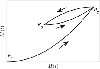
In magnetic hysteresis, when magnetization M is plotted against magnetic field H the following is observed. The curve (H(t),M(t))(H(t),M(t)) follows the path P1P2P1P2 when H increases with time t (see Fig. 2). Then the path P2P3P2P3 is followed when H decreases. What is important to note is that, when H increases again from the point P3P3, the path followed by (H(t),M(t))(H(t),M(t)) ends precisely at the pointP2P2 (see for example Ref. [31]).
Fig. 2

The path P1P2P1P2 is part of the major loop. The path P2P3P2P2P3P2 is a minor loop.

The loop formed by the path P2P3P2P2P3P2 is called a minor loop. It occurs in electromagnetic devices when the input is periodic but not exactly sinusoidal. The distortion of the input generates minor loops when hysteresis is involved which causes energy losses. This fact explains the interest of analyzing the behavior of minor loops.

In what follows we formalize mathematically the behavior observed in Fig. 2.

Let umin,1,umin,2,umax,1,umax,2Rumin,1,umin,2,umax,1,umax,2R such that umin,1umin,2<umax,1umax,2umin,1umin,2<umax,1umax,2 and at least one of the following holds: umin,1umin,2umin,1umin,2 or umax,1umax,2umax,1umax,2. Let α1,α2,α3,TRα1,α2,α3,TR with 0<α1<α2<α3<T0<α1<α2<α3<T. Consider a T–periodic input u:R+[umin,1,umax,2]u:R+[umin,1,umax,2] such that
  1. (i)

    the function u is continuous on R+R+,

     
  2. (ii)

    the function u is continuously differentiable on ]0,α1[]0,α1[, ]α1,α2[]α1,α2[, ]α2,α3[]α2,α3[, and ]α3,T[]α3,T[ with ˙u<u˙<,

     
  3. (iii)

    the function u is strictly increasing on ]0,α1[]0,α1[, strictly decreasing on ]α1,α2[]α1,α2[, strictly increasing on ]α2,α3[]α2,α3[, and strictly decreasing on ]α3,T[]α3,T[,

     
  4. (iv)

    we have u(0)=u(T)=umin,1u(0)=u(T)=umin,1, u(α1)=umax,1u(α1)=umax,1, u(α2)=umin,2u(α2)=umin,2, u(α3)=umax,2u(α3)=umax,2.

     
Let Mumin,1,umin,2,umax,1,umax,2,α1,α2,α3,TMumin,1,umin,2,umax,1,umax,2,α1,α2,α3,T be the set of all such inputs u, and let ΞΞ be a set of initial conditions. In this section, we consider an operator H:W1,(R+,R)×ΞL(R+,Rm)C0(R+,Rm)H:W1,(R+,R)×ΞL(R+,Rm)C0(R+,Rm) that is causal and that satisfies Assumption 3. We assume that HH is consistent with respect to all (u,x0)W1,(R+,R)×Ξ(u,x0)W1,(R+,R)×Ξ and is strongly consistent with respect to all periodic inputs uW1,(R+,R)uW1,(R+,R) and all initial states x0Ξx0Ξ.
For uMumin,1,umin,2,umax,1,umax,2,α1,α2,α3,TuMumin,1,umin,2,umax,1,umax,2,α1,α2,α3,T define ϱi=ρu(αi),i=1,2,3ϱi=ρu(αi),i=1,2,3. Then we have
ϱ1=umax,1umin,1,
ϱ1=umax,1umin,1,
(53)
ϱ2=ϱ1+umax,1umin,2,
ϱ2=ϱ1+umax,1umin,2,
(54)
ϱ3=ϱ2+umax,2umin,2,
ϱ3=ϱ2+umax,2umin,2,
(55)
ρu(T)=ϱ4=ϱ3+umax,2umin,1.
(56)
The function ψuW1,(R+,R)ψuW1,(R+,R) in ϱ4ϱ4–periodic by Lemma 5, and can be determined using Lemma 1 as
ψu(ϱ)=ϱ+umin,1,ϱ[0,ϱ1],
(57)
ψu(ϱ)=ϱ+ϱ1+umax,1,ϱ[ϱ1,ϱ2],
(58)
ψu(ϱ)=ϱϱ2+umin,2,ϱ[ϱ2,ϱ3],
(59)
ψu(ϱ)=ϱ+ϱ3+umax,2,ϱ[ϱ3,ϱ4].
(60)
Define
ϱ5=umax,1umin,2+ϱ2]ϱ2,ϱ3],ϱ6=umin,2umin,1]0,ϱ1[,ϱ7=ϱ3+umax,2umin,2]ϱ3,ϱ4[.
ϱ5=ϱ6=ϱ7=umax,1umin,2+ϱ2]ϱ2,ϱ3],umin,2umin,1]0,ϱ1[,ϱ3+umax,2umin,2]ϱ3,ϱ4[.
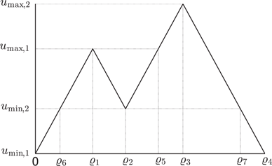
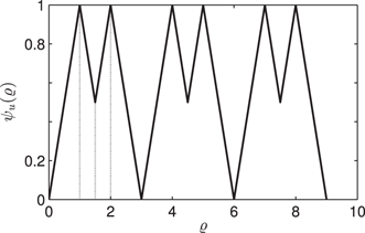
Then ψu(ϱ1)=ψu(ϱ5)=umax,1ψu(ϱ1)=ψu(ϱ5)=umax,1 and ψu(ϱ2)=ψu(ϱ6)=ψ(ϱ7)=umin,2ψu(ϱ2)=ψu(ϱ6)=ψ(ϱ7)=umin,2. Figure 3 illustrates what has been exposed up till now.
Fig. 3

ψu(ϱ)ψu(ϱ) versus ϱϱ.

Assumption 8

(u,x0)Mumin,1,umin,2,umax,1,umax,2,α1,α2,α3,T×Ξ(u,x0)Mumin,1,umin,2,umax,1,umax,2,α1,α2,α3,T×Ξ we have φu(ϱ1)=φu(ϱ5)φu(ϱ1)=φu(ϱ5).

Definition 11

Under Assumption 8 define the sets
Vu={(ψu(ϱ),φu(ϱ)),ϱ[0,ϱ1][ϱ5,ϱ4]},
(61)
Nu={(ψu(ϱ),φu(ϱ)),ϱ[ϱ1,ϱ5]}.
(62)
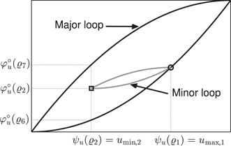
The set VuVu is called the major loop and the set NuNu a minor loop (see Fig. 4).
Depending on the particular field in which hysteresis is observed, minor loops may have some additional properties that may be formalized mathematically. As an example, for magnetic hysteresis Assumption 8 holds [31], and we observe that if umax,1<umax,2umax,1<umax,2 then for all (u,x0)Mumin,1,umin,2,umax,1,umax,2,α1,α2,α3,T×Ξ(u,x0)Mumin,1,umin,2,umax,1,umax,2,α1,α2,α3,T×Ξ, Properties (i)–(ii) hold.
  1. (i)

    VuNu={(ψu(ϱ1),φu(ϱ1))=(ψu(ϱ5),φu(ϱ5))}.VuNu={(ψu(ϱ1),φu(ϱ1))=(ψu(ϱ5),φu(ϱ5))}.

     
  2. (ii)

    φu(ϱ6)<φu(ϱ2)<φu(ϱ7)φu(ϱ6)<φu(ϱ2)<φu(ϱ7) or φu(ϱ7)<φu(ϱ2)<φu(ϱ6)φu(ϱ7)<φu(ϱ2)<φu(ϱ6).

     
Property (i) says that the major loop and the minor loop intersect at only one point when umax,1<umax,2umax,1<umax,2. Property (ii) says that the minor loop is located inside the major loop. Both conditions are the transcription of experimental observations in magnetic hysteresis (see for example [4, Fig. 7]).
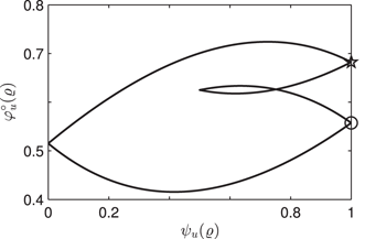
Note that the hysteresis loop GuGu of Equation (31) is such that Gu=VuNuGu=VuNu. Figure 4 provides an example of a minor loop and a major loop that correspond to the normalized input of Figure 3.
Fig. 4

Hysteresis loop φu(ϱ)φu(ϱ) versus ψu(ϱ)ψu(ϱ) for ϱ[0,ϱ4].ϱ[0,ϱ4]. Black: major loop Vu.Vu. Grey: minor loop Nu.Nu. The marker open circle corresponds to the point (ψu(ϱ1),φu(ϱ1))=(ψu(ϱ5),φu(ϱ5)).(ψu(ϱ1),φu(ϱ1))=(ψu(ϱ5),φu(ϱ5)). The marker rectangle corresponds to the point (ψu(ϱ2),φu(ϱ2)).(ψu(ϱ2),φu(ϱ2)).

The concepts introduced in this section are applied to the scalar semilinear Duhem model in Sect. 11.9.

11 Case Study: The Semilinear Duhem Model

In this section we use the semilinear Duhem model to illustrate the concepts presented in this paper, and to analyze the relationships between these concepts. Section 11.1 presents the model. In Sect. 11.2 we provide sufficient conditions for the consistency of the model. Section 11.3 focuses on the study of the strong consistency of the semilinear Duhem model. The results of Sects. 11.2 and 11.3 are illustrated by numerical simulations in Sect. 11.4. In Sect. 11.5 we specialize into the scalar version of the semilinear Duhem model. Section 11.5 provides the conditions under which the scalar semilinear Duhem model is a hysteresis according to Definition 4. The results of Sect. 11.5 are illustrated by numerical simuations in Sect. 11.6. The relationship between Definition 4 and strong consistency is commented upon in Sect. 12.1. Section 11.7 analyzes the dissipativity of the scalar rate-independent semilinear Duhem model. The results of Sect. 11.7 are illustrated by numerical simulations in Sect. 11.8. The relationship between dissipativity and orientation of the hysteresis loop is commented upon in Sect. 12.3. The minor loops of the scalar semilinear Duhem model are studied and commented upon in Sect. 11.9.

11.1 The Semilinear Duhem Model: Definition and Global Existence of Solutions

The semilinear Duhem model is a special case of the generalized Duhem model (17)–(19). It is called so because, although the model may be nonlinear with respect to the input, the state appears linearly both in the state equation (63) and in the output equation (65). The semilinear Duhem model has been proposed in Ref. [54] as:
˙x(t)=g1(˙u(t))(A1x(t)+B1u(t)+E1)+g2(˙u(t))(A2x(t)+B2u(t)+E2) for  almost  all tR+,
x˙(t)=g1(u˙(t))(A1x(t)+B1u(t)+E1)+g2(u˙(t))(A2x(t)+B2u(t)+E2) for  almost  all tR+,
(63)
x(0)=x0,
x(0)=x0,
(64)
y(t)=Cx(t)+Du(t),tR+.
(65)
In Eqs. (63)–(65) the matrix A1Rn×nA1Rn×n where n is a strictly positive integer, A2Rn×n,A2Rn×n,B1Rn×1,B1Rn×1,B2Rn×1,B2Rn×1,E1Rn×1,E1Rn×1,E2Rn×1,E2Rn×1,CR1×n,CR1×n, and DR.DR. We consider that C(0,,0)C(0,,0) to avoid having a linear process y=Duy=Du that does not describe hysteresis. We consider that uW1,(R+,R)uW1,(R+,R) whereas the properties of y:R+Ry:R+R and x:R+Rnx:R+Rn will be analyzed in Theorem 5. The functions g1:RRg1:RR and g2:RRg2:RR are continuous and satisfy g1(w)=0g1(w)=0 for w0,w0,g2(w)=0g2(w)=0 for w0w0. Define
ˉg1(w)=g1(w)|w|,w0,
g¯1(w)=g1(w)|w|,w0,
(66)
ˉg2(w)=g2(w)|w|,w0.
g¯2(w)=g2(w)|w|,w0.
(67)
As in Ref. [54] we assume that20
limw0ˉg1(w)=1 and limw0ˉg2(w)=1.
limw0g¯1(w)=1 and limw0g¯2(w)=1.
(68)
In Eq. (63), the functions g1(˙u)g1(u˙) and g2(˙u)g2(u˙) are measurable [60, Theorem 1.12(d)]. Thus, the differential equation (63) can be seen as a linear time-varying system that satisfies all the assumptions of [29, Theorem 3]. This implies that a unique absolutely continuous solution of (63) exists on R+R+.

As noted in Ref. [54], the semilinear Duhem model is rate independent when g1(w)=max(0,w)g1(w)=max(0,w) and g2(w)=min(0,w),wRg2(w)=min(0,w),wR.

11.2 Consistency of the Semilinear Duhem Model

This section presents the results obtained in Ref. [35] in relation with the consistency of the semilinear Duhem model.

Theorem 5

[35] Consider the semilinear Duhem model (63)–(65). Assume that both matricesA1A1 andA2A2 are stable21 and have a common Lyapunov matrixP=PT>0P=PT>0 (that isAT1P+PA1<0AT1P+PA1<0 andAT2PPA2<0AT2PPA2<0). Then, xW1,(R+,Rn)xW1,(R+,Rn) andyW1,(R+,R)yW1,(R+,R).

In Eqs. (63)–(65) consider the operators Hs:L(R+,R)×W1,(R+,R)×RnW1,(R+,R)Hs:L(R+,R)×W1,(R+,R)×RnW1,(R+,R) and Ho:L(R+,R)×W1,(R+,R)×RnW1,(R+,R)Ho:L(R+,R)×W1,(R+,R)×RnW1,(R+,R) such that Hs(˙u,u,x0)=xHs(u˙,u,x0)=x, and Ho(˙u,u,x0)=yHo(u˙,u,x0)=y.

Observe that the operators HsHs and HoHo are causal owing to the uniqueness of the solutions of (63)–(64).

Consider the left-derivative operator ΔΔ defined on W1,(R+,R)W1,(R+,R) by [Δ(u)](t)=limτtu(τ)u(t)τt[Δ(u)](t)=limτtu(τ)u(t)τt. The operator ΔΔ is causal as [Δ(u)](t)[Δ(u)](t) depends only on the values of u(τ)u(τ) for τtτt. We also have Δ(u)=˙uΔ(u)=u˙ almost everywhere since uW1,(R+,R)uW1,(R+,R) so that Δ(u)L(R+,R)Δ(u)L(R+,R), that is Δ:W1,(R+,R)L(R+,R)Δ:W1,(R+,R)L(R+,R).

Consider the operators Hs,Ho:W1,(R+,R)×RnW1,(R+,R)Hs,Ho:W1,(R+,R)×RnW1,(R+,R) defined by the relations
Hs(u,x0)=Hs(Δ(u),u,x0)=x,Ho(u,x0)=Ho(Δ(u),u,x0)=y.
Hs(u,x0)=Ho(u,x0)=Hs(Δ(u),u,x0)=x,Ho(Δ(u),u,x0)=y.
Then HsHs and HoHo are causal. Observe also that HsHs and HoHo satisfy Assumption 3. These facts mean the the operators HsHs and HoHo belong to the class of operators of Sect. 6.2 so that the definitions and results of Sects. 6.36.5 apply.
To study the consistency of the operators HsHs and HoHo we follow the steps given in Sect. 6.4. If instead of u the input is usγusγ where γ]0,[γ]0,[ then Eq. (63) becomes
˙xγ(t)=g1(˙uγ(t))(A1xγ(t)+B1uγ(t)+E1)+g2(˙uγ(t))(A2xγ(t)+B2uγ(t)+E2) for  almost  all t0
x˙γ(t)=g1(u˙γ(t))(A1xγ(t)+B1uγ(t)+E1)+g2(u˙γ(t))(A2xγ(t)+B2uγ(t)+E2) for  almost  all t0
(69)
where uγ=usγuγ=usγ. The initial state remains the same for all γγ as explained in Sect. 6.4 so that Eq. (64) becomes
xγ(0)=x0.
xγ(0)=x0.
(70)
Given ϱIuϱIu there exists a not necessarily unique tϱ,γR+tϱ,γR+ such that ρusγ(tϱ,γ)=ϱρusγ(tϱ,γ)=ϱ. Since the operator HsHs belongs to the class of operators of Sect. 6.2 it follows that xγ(tϱ,γ)xγ(tϱ,γ) is independent of the particular choice of tϱ,γtϱ,γ [35]. Thus, a function xusγ:IuRnxusγ:IuRn can be defined by the relation xusγ(ϱ)=xγ(tϱ,γ)xusγ(ϱ)=xγ(tϱ,γ) so that xusγρusγ=xγxusγρusγ=xγ (recall that by Lemma 2 we have Iusγ=IuIusγ=Iu). We call the function xusγxusγ the normalized state.
Also, if instead of u the input is usγusγ then Eq. (65) becomes
yγ(t)=Cxγ(t)+Dusγ(t),tR+.
(71)
Given ϱIuϱIu there exists a not necessarily unique tϱ,γR+tϱ,γR+ such that ρusγ(tϱ,γ)=ϱρusγ(tϱ,γ)=ϱ. Since the operator HoHo belongs to the class of operators of Sect. 6.2 it follows that yγ(tϱ,γ)yγ(tϱ,γ) is independent of the particular choice of tϱ,γtϱ,γ. Thus, the normalized output φusγ:IuRnφusγ:IuRn is defined by the relation φusγ(ϱ)=yγ(tϱ,γ)φusγ(ϱ)=yγ(tϱ,γ) so that φusγρusγ=yγφusγρusγ=yγ. Taking into account that ψusγ=ψuψusγ=ψu by Lemma 2 we get
φuγ(ϱ)=Cxuγ(ϱ)+Dψu(ϱ),ϱIu.
(72)
Finally, given ϱIuϱIu there exists a not necessarily unique tϱR+tϱR+ such that ρu(tϱ)=ϱρu(tϱ)=ϱ. Since the operator ΔΔ belongs to the class of operators of Sect. 6.2 it follows that ˙u(tϱ)u˙(tϱ) is independent of the particular choice of tϱtϱ. This implies that a function vu:IuRvu:IuR can be defined almost everywhere by the relation vu(ϱ)=˙u(tϱ)vu(ϱ)=u˙(tϱ). The function vuL(Iu,R)vuL(Iu,R) by Lemma 3 and we have vuρu=˙uvuρu=u˙. We call function vuvu the normalized input-derivative. More about vuvu in 16.

Theorem 6

[35] Consider the semilinear Duhem model (63)–(65). Assume that both matricesA1A1 andA2A2 are stable and have a common Lyapunov matrixP=PT>0.P=PT>0. Then, for allγ]0,[,γ]0,[,xusγW1,(R+,Rn)xusγW1,(R+,Rn) andφusγW1,(Iu,R).φusγW1,(Iu,R). Moreover
xusγ(σ)=x0+σ0ˉg1(vu(ϱ)γ)[A1xusγ(ϱ)+B1ψu(ϱ)+E1]+ˉg2(vu(ϱ)γ)[A2xusγ(ϱ)+B2ψu(ϱ)+E2]dϱ,σIu.
xusγ(σ)=x0+σ0g¯1(vu(ϱ)γ)[A1xusγ(ϱ)+B1ψu(ϱ)+E1]+g¯2(vu(ϱ)γ)[A2xusγ(ϱ)+B2ψu(ϱ)+E2]dϱ,σIu.
(73)
Also !xuW1,(Iu,Rn)!xuW1,(Iu,Rn) such that limγxuxusγIu=0limγxuxusγIu=0 which means that the operator HsHs is consistent with respect to all (u,x0)W1,(R+,Rn)×Rn(u,x0)W1,(R+,Rn)×Rn; and !φuW1,(Iu,R)!φuW1,(Iu,R) such that limγφuφusγIu=0limγφuφusγIu=0 which means that the operator HoHo is consistent with respect to all (u,x0)W1,(R+,Rn)×Rn(u,x0)W1,(R+,Rn)×Rn. We have:
dxudϱ(ϱ)=˙ψu(ϱ)+12(A1xu(ϱ)+B1ψu(ϱ)+E1)+˙ψu(ϱ)12(A2xu(ϱ)+B2ψu(ϱ)+E2) for almost all ϱIu,
dxudϱ(ϱ)=ψ˙u(ϱ)+12(A1xu(ϱ)+B1ψu(ϱ)+E1)+ψ˙u(ϱ)12(A2xu(ϱ)+B2ψu(ϱ)+E2) for almost all ϱIu,
(74)
xu(0)=x0,
xu(0)=x0,
(75)
φu(ϱ)=Cxu(ϱ)+Dψu(ϱ),ϱIu.
(76)

11.3 Strong Consistency of the Semilinear Duhem Model

This section presents the results obtained in Ref. [35] in relation with the strong consistency of the semilinear Duhem model.

To study the strong consistency of the operators HsHs and HoHo we follow the steps given in Sect. 6.5. Consider an input u that is non constant and T–periodic where T]0,[T]0,[. For any nonnegative integer k, define xu,kW1,([0,ρu(T)],Rm)xu,kW1,([0,ρu(T)],Rm) by
xu,k(ϱ)=xu(ρu(T)k+ϱ),ϱ[0,ρu(T)],
(77)
and define φu,kW1,([0,ρu(T)],Rm)φu,kW1,([0,ρu(T)],Rm) by
φu,k(ϱ)=φu(ρu(T)k+ϱ),ϱ[0,ρu(T)].
(78)

Theorem 7

[35] Consider the semilinear Duhem model (63)–(65). Assume that the matricesA1A1 andA2A2 are both stable and have a common Lyapunov matrixP=PT>0P=PT>0. Let(u,x0)W1,(R+,Rn)×Rn(u,x0)W1,(R+,Rn)×Rn be such thatu is non constant andTperiodic. Then there exists a unique functionxuW1,([0,ρu(T)],Rn)xuW1,([0,ρu(T)],Rn) such thatlimkxu,kxu[0,ρu(T)]=0limkxu,kxu[0,ρu(T)]=0 which means that the operatorHsHs is strongly consistent with respect to(u,x0)(u,x0). Also!φuW1,([0,ρu(T)],R)!φuW1,([0,ρu(T)],R) such thatlimkφu,kφu[0,ρu(T)]=0limkφu,kφu[0,ρu(T)]=0 which means that the operatorHoHo is strongly consistent with respect to(u,x0)(u,x0). We havexu(0)=xu(ρu(T))xu(0)=xu(ρu(T)), φu(0)=φu(ρu(T)),φu(0)=φu(ρu(T)), and
dxudϱ(ϱ)=˙ψu(ϱ)+12(A1xu(ϱ)+B1ψu(ϱ)+E1)+˙ψu(ϱ)12(A2xu(ϱ)+B2ψu(ϱ)+E2) for almost all ϱ[0,ρu(T)],
dxudϱ(ϱ)=ψ˙u(ϱ)+12(A1xu(ϱ)+B1ψu(ϱ)+E1)+ψ˙u(ϱ)12(A2xu(ϱ)+B2ψu(ϱ)+E2) for almost all ϱ[0,ρu(T)],
(79)
φu(ϱ)=Cxu(ϱ)+Dψu(ϱ),ϱ[0,ρu(T)].
(80)
Note that the initial condition xu(0)xu(0) may be different from x0x0.

Special cases22

Special case 1. We consider that uΛumin,umax,α1,TuΛumin,umax,α1,T (see Equation (20)). In this case it is possible to find the explicit expression for the initial condition xu(0)xu(0). Indeed, from Eq. (79) it comes that
dxudϱ(ϱ)=A1xu(ϱ)+B1ψu(ϱ)+E1,ϱ]0,ρu(α1)[.
(81)
The differential equation (81) gives
xu(ρu(α1))=eρu(α1)A1xu(0)+eρu(α1)A1ρu(α1)0eϱA1(B1ψu(ϱ)+E1)dϱ.
(82)
On the other hand, using Lemma 1 and the fact that uΛumin,umax,α1,TuΛumin,umax,α1,T it comes that
ψu(ϱ)=ϱ+umin,ϱ[0,ρu(α1)],
(83)
ψu(ϱ)=ϱ+2umaxumin,ϱ[ρu(α1),ρu(T)],
(84)
ρu(α1)=umaxumin,
ρu(α1)=umaxumin,
(85)
ρu(T)=2(umaxumin).
ρu(T)=2(umaxumin).
(86)
Combining Eqs. (83), (82) and (85) we get
xu(umaxumin)=e(umaxumin)A1xu(0)+(A11(umaxumin)A21+A21e(umaxumin)A1)B1+(A11+A11e(umaxumin)A1)×(B1umin+E1).
(87)
Note that the matrix A1A1 is invertible as it is stable. Also, the differential equation (79) gives
xu(ρu(T))=e(ρu(T)ρu(α1))A2xu(ρu(α1))eρu(T)A2ρu(T)ρu(α1)eϱA2(B2ψu(ϱ)+E2)dϱ.
(88)
Combining Eqs. (84)–(88) it comes that
xu(2(umaxumin))=e(uminumax)A2xu(umaxumin)+B2[A22+2(umaxumin)A12+A22e(uminumax)A2A12e(uminumax)A2(umaxumin)]+(A12+A12e(uminumax)A2)×(B2(2umaxumin)+E2).
(89)
Note that the matrix A2A2 is invertible as A2A2 is stable. From Theorem 7 it follows that that xu(2(umaxumin))=xu(0)xu(2(umaxumin))=xu(0) owing to Eq. (86). This equality combined with Eqs. (89) and (87) gives
xu(0)=θ=D10N0,N0=e(uminumax)A2[(A11(umaxumin)A21+A21e(umaxumin)A1)B1+(A11+A11e(umaxumin)A1)(B1umin+E1)]+[A22+2(umaxumin)A12+A22e(uminumax)A2A12e(uminumax)A2(umaxumin)]B2+(A12+A12e(uminumax)A2)×(B2(2umaxumin)+E2),D0=Ine(uminumax)A2e(umaxumin)A1,
xu(0)N0=D0==θ=D10N0,e(uminumax)A2[(A11(umaxumin)A21+A21e(umaxumin)A1)B1+(A11+A11e(umaxumin)A1)(B1umin+E1)]+[A22+2(umaxumin)A12+A22e(uminumax)A2A12e(uminumax)A2(umaxumin)]B2+(A12+A12e(uminumax)A2)×(B2(2umaxumin)+E2),Ine(uminumax)A2e(umaxumin)A1,
(90)
where InIn is the n×nn×n identity matrix.

Special case 2. We consider that uΛumin,umax,α1,TuΛumin,umax,α1,T and n=1n=1. Our aim is to study the conditions for which the hysteresis loop of the scalar semilinear Duhem model is not trivial (see Definition 9).

To this end, combining Eqs. (81), (83) and (85) we get
˙ξ1(ν)=A1ξ1(ν)+B1ν+E1,ν]umin,umax[,
ξ˙1(ν)=A1ξ1(ν)+B1ν+E1,ν]umin,umax[,
(91)
where ξ1:[umin,umax]Rξ1:[umin,umax]R is defined by the relation ξ1(ν)=xu(ϱ)ξ1(ν)=xu(ϱ) with ν=ϱ+uminν=ϱ+umin and ϱ[0,ρu(α1)]ϱ[0,ρu(α1)]. Similarly, for ϱ[ρu(α1),ρu(T)]ϱ[ρu(α1),ρu(T)] we get
˙ξ2(ν)=A2ξ2(ν)+B2ν+E2,ν]umin,umax[,
ξ˙2(ν)=A2ξ2(ν)+B2ν+E2,ν]umin,umax[,
(92)
where ξ2:[umin,umax]Rξ2:[umin,umax]R is defined by the relation ξ2(ν)=xu(ϱ)ξ2(ν)=xu(ϱ) with ν=ϱ+2umaxuminν=ϱ+2umaxumin.
Solving the differential equations (91) and (92) we get for all ν[umin,umax]ν[umin,umax]
ξ1(ν)=B1A1νE1A1B1A21+(B1A1umin+E1A1+B1A21+θ)eA1(νumin),
(93)
ξ2(ν)=B2A2νE2A2B2A22+(B2A2umin+E2A2+B2A22+θ)eA2(νumin).
(94)
The hysteresis loop GuGu of the operator HoHo with respect to (u,x0)(u,x0) is independent of the initial state x0x0 and is given by (see Definition 8):
Gu={(ν,Cξ1(ν)+Dν),ν[umin,umax]}{(ν,Cξ2(ν)+Dν),ν[umin,umax]}.
(95)

Lemma 8

Consider the semilinear Duhem model (63)–(65) with n=1n=1, A1<0A1<0 andA2>0A2>0. Then, Propositions (i) and (ii) are equivalent.
  1. (i)

    For all (u,x0)Λumin,umax,α1,T×R(u,x0)Λumin,umax,α1,T×R, the operator HoHo has a trivial hysteresis loop with respect to (u,x0)(u,x0).

     
  2. (ii)
    Equalities (96) and (97) hold.
    A12B2=A11B1,
    A12B2=A11B1,
    (96)
    B1A11(A12A11)E1A11+E2A12=0.
    B1A11(A12A11)E1A11+E2A12=0.
    (97)
     

Proof

See Appendix 19.

11.4 Illustration of the Consistency and Strong Consistency of the Scalar Semilinear Duhem Model

We consider the semilinear Duhem model with the following parameters: n=1,n=1,A1=1,A1=1,A2=1,A2=1,B1=1,B1=1,B2=1,B2=1,E1=0,E1=0,E2=0,E2=0,C=1,C=1,D=0.D=0. The function g1:RRg1:RR is defined by the relations xR,g1(x)=0xR,g1(x)=0 if x0x0, and g1(x)=x+x2g1(x)=x+x2 if x0x0. The function g2:RRg2:RR is defined by the relations xR,g2(x)=0xR,g2(x)=0 if x0x0, and g2(x)=xg2(x)=x if x0x0.

Consider the 2–periodic input u defined as follows: u(t)=t,t[0,1]u(t)=t,t[0,1], and u(t)=2t,t[1,2]u(t)=2t,t[1,2] (see Fig. 5).
Fig. 5

u(t) versus t.

Observe that, since ρuρu is the identity function, we have vu=˙uvu=u˙ almost everywhere so that in the differential equation (73) we have vu(ϱ)=1,ϱ]0,1[vu(ϱ)=1,ϱ]0,1[ and vu(ϱ)=1,ϱ]1,2[vu(ϱ)=1,ϱ]1,2[. The following values of γγ are considered: γ=1γ=1, γ=10γ=10 and γ=100γ=100. The differential equation (73) is solved using Matlab solver ode23s for the three values of γγ and with the initial condition x0=0x0=0. For each value of γγ we obtain the corresponding xuγxuγ which, in this case, is equal to φuγφuγ as C=1C=1 and D=0D=0 [see Eq. (72)]. Figure 6 provides the plot of function φuγ(ϱ)φuγ(ϱ) versus time ϱϱ for γ=1γ=1, γ=10γ=10 and γ=100γ=100 (dotted). The same figure provides the plot of function φu(ϱ)φu(ϱ) versus time ϱϱ (solid). The plot of φuφu has been obtained by solving the differential equation (74) using Matlab solver ode23s, and taking into account that ψu=uψu=u and that the initial condition φu(0)φu(0) is also x0=0x0=0 [see Eq. (75)]. Since C=1C=1 and D=0D=0 we have φu=xuφu=xu [see Eq. (76)]. We can see that the plots φuγ(ϱ)φuγ(ϱ) versus ϱϱ converge to the plot φu(ϱ)φu(ϱ) versus ϱϱ as γγ increases which is predicted by Theorem 6.
Fig. 6

Dotted: φusγ(ϱ)φusγ(ϱ) versus ϱϱ for γ=1γ=1, γ=10γ=10 and γ=100γ=100. Solid: φu(ϱ)φu(ϱ) versus ϱϱ (labeled as γ=γ=). Note that the plot that corresponds to γ=100γ=100 is practically equal to the one that corresponds to γ=γ=.

Now that φuφu has been computed, the functions φu,kφu,k where kNkN are determined using Eq. (78). Figure 7 provides the plots of function φu,k(ϱ)φu,k(ϱ) versus ϱϱ for k=0k=0, k=1k=1 and k=2k=2 (dotted). The same figure provides the plot of the function φu(ϱ)φu(ϱ) versus time ϱϱ (solid). The plot of φuφu is obtained by solving the differential equation (79) using Matlab solver ode23s, and taking into account that ψu=uψu=u. The initial condition xu(0)xu(0) is obtained from Eq. (90). Note that we have φu=xuφu=xu as C=1C=1 and D=0D=0 (see Eq. (80)). As predicted by Theorem 7 it can be seen that the plots φu,k(ϱ)φu,k(ϱ) versus ϱϱ converge to the plot φu(ϱ)φu(ϱ) versus ϱϱ as k increases.
Fig. 7

Dotted: φu,k(ϱ)φu,k(ϱ) versus ϱϱ for k=0k=0, k=1k=1 and k=2k=2. Solid: φu(ϱ)φu(ϱ) versus ϱϱ (labeled as k=k=). Note that the plot that corresponds to k=2k=2 is practically equal to the one that corresponds to k=k=.

The hysteresis loop of the operator HoHo with respect to (u,x0)(u,x0), that is the set {(ψu(ϱ),φu(ϱ)),ϱ[0,2]}{(ψu(ϱ),φu(ϱ)),ϱ[0,2]} (see Eq. (31)), is plotted in Fig. 8. It can be seen that the hysteresis loop is not trivial as predicted by Lemma 8 since Equality (97) does not hold.
Fig. 8

φu(ϱ)φu(ϱ) versus ψu(ϱ)ψu(ϱ) for ϱ[0,2]ϱ[0,2].

We now use the value E2=2E2=2 instead of E2=0E2=0 so that both Equalities (96) and (97) hold. Lemma 8 predicts that the hysteresis loop is trivial as can be observed in Fig. 9.
Fig. 9

φu(ϱ)φu(ϱ) versus ψu(ϱ)ψu(ϱ) for ϱ[0,2]ϱ[0,2].

11.5 Hysteresis Property -According to Definition 4- of the Scalar Semilinear Duhem Model

In this section we focus on the scalar version of the semilinear Duhem model (63)–(65), that is we consider that n=1n=1. We also consider that A1<0A1<0 and A2>0A2>0 so that Theorem 5 applies.

Our aim is to check whether the scalar semilinear Duhem model is a hysteresis according to Definition 4. To this end, we need to check whether Assumptions 1 and 2 hold as a prerequisite for Definition 4. Owing to Theorem 5 we can see that xW1,(R+,R)xW1,(R+,R) so that Assumption 1 is satisfied.

Now, we have to check whether Assumption 2 is satisfied. To this end, let γ]0,[γ]0,[ and uΛumin,umax,α1,TuΛumin,umax,α1,T; recall that the input usγusγ is TγTγ–periodic where sγsγ is a linear time-scale change. Assumption 2 will be satisfied if we can find a unique initial condition x0,γRx0,γR such that Hs(usγ,x0,γ)Hs(usγ,x0,γ) is also TγTγ–periodic.

When the semilinear Duhem model is rate independent, x0,γx0,γ is independent of γγ. In this case Ref. [54] provides the expression of x0,γx0,γ (see [54, Eqs. (4.9)–(4.14)]) which means that Assumption 2 is satisfied.

However, Ref. [54] provides no proof that Assumption 2 is satisfied for the rate-dependent semilinear Duhem model. Instead, another argument is used in the proof of [54, Proposition 5.1] to check whether the rate-dependent semilinear Duhem model is a hysteresis according to Definition 4 (or equivalently [54, Definition 2.2]). As shown in Section 12.1.3, that argument does not imply necessarily that Assumption 2 is satisfied.

In what follows we prove that Assumption 2 is satisfied for both the rate-independent and the rate-dependent scalar semilinear Duhem model.

Theorem 8

Consider the semilinear Duhem model (63)–(65) withn=1n=1, A1<0A1<0, A2>0A2>0. LetuΛumin,umax,α1,TuΛumin,umax,α1,T. Then, γ0>0γ0>0 such thatγ]γ0,[γ]γ0,[ there exists a uniquex0,γRx0,γR such thatHs(usγ,x0,γ)Hs(usγ,x0,γ) is alsoTγTγperiodic.

Proof

See Appendix 17.

Theorem 8 shows that Assumption 2 is satisfied (see Remark 1). Our objective now is to prove that Conditions (i) and (ii) of Definition 4 are met. We start with Condition (i).

The authors of Ref. [54] provide no proof that Condition (i) of Definition 4 is satisfied for the rate-dependent semilinear Duhem model (for the rate-independent model, the proof is trivial). To prove that Condition (i) is met we start by finding the explicit expression of the set Cu,γCu,γ of Equation (21). Let γ]γ0,[γ]γ0,[ where γ0γ0 is given by Eq. (139). From Eqs. (21) and (169) it follows that
Cu,γ={(u(σ),Cˉzγ(σ)+Du(σ)),σ[0,T]}.
Cu,γ={(u(σ),Cz¯γ(σ)+Du(σ)),σ[0,T]}.
(98)
where ˉzγz¯γ is defined in Appendix 17, Eq. (166).
Define the function h1:[0,α1]Rh1:[0,α1]R by
h1(σ)=(ˉzγ(0)+σ0γg1(˙u(τ)γ)(B1u(τ)+E1)exp(γA1τ0g1(˙u(t)γ)dt)dτ)×exp(γA1σ0g1(˙u(τ)γ)dτ),σ[0,α1].
h1(σ)=z¯γ(0)+σ0γg1(u˙(τ)γ)(B1u(τ)+E1)exp(γA1τ0g1(u˙(t)γ)dt)dτ×exp(γA1σ0g1(u˙(τ)γ)dτ),σ[0,α1].
(99)
It can be checked that h1h1 satisfies the following differential equation
˙h1(σ)=γg1(˙u(τ)γ)(A1h1(σ)+B1u(σ)+E1),σ]0,α1[,h1(0)=ˉzγ(0).
h˙1(σ)h1(0)=γg1(u˙(τ)γ)(A1h1(σ)+B1u(σ)+E1),σ]0,α1[,=z¯γ(0).
(100)
Owing to the uniqueness of the solutions of (167) it comes that
ˉzγ(σ)=h1(σ),σ[0,α1].
z¯γ(σ)=h1(σ),σ[0,α1].
(101)
A similar argument on the interval [α1,T][α1,T] shows that
ˉzγ(σ)=(ˉzγ(α1)+σα1γg2(˙u(τ)γ)(B2u(τ)+E2)exp(γA2τα1g2(˙u(t)γ)dt)dτ)×exp(γA2σα1g2(˙u(τ)γ)dτ),σ[α1,T].
z¯γ(σ)=z¯γ(α1)+σα1γg2(u˙(τ)γ)(B2u(τ)+E2)exp(γA2τα1g2(u˙(t)γ)dt)dτ×exp(γA2σα1g2(u˙(τ)γ)dτ),σ[α1,T].
(102)
Owing to the T–periodicity of ˉzγz¯γ we have ˉzγ(T)=ˉzγ(0)z¯γ(T)=z¯γ(0). This fact along with Eqs. (99), (101), and (102) gives
ˉzγ(0)=x0,γ=ND,
z¯γ(0)=x0,γ=ND,
(103)
where
N=exp[α10γA1g1(˙u(τ)γ)dτ+Tα1γA2g2(˙u(τ)γ)dτ]×α10γg1(˙u(τ)γ)(B1u(τ)+E1)exp(γA1τ0g1(˙u(t)γ)dt)dτ+exp[γA2Tα1g2(˙u(τ)γ)dτ]×Tα1γg2(˙u(τ)γ)(B2u(τ)+E2)exp(γA2τα1g2(˙u(t)γ)dt)dτ,D=1exp[γA1α10g1(˙u(τ)γ)dτ+γA2Tα1g2(˙u(τ)γ)dτ].
N=D=exp[α10γA1g1(u˙(τ)γ)dτ+Tα1γA2g2(u˙(τ)γ)dτ]×α10γg1(u˙(τ)γ)(B1u(τ)+E1)exp(γA1τ0g1(u˙(t)γ)dt)dτ+exp[γA2Tα1g2(u˙(τ)γ)dτ]×Tα1γg2(u˙(τ)γ)(B2u(τ)+E2)exp(γA2τα1g2(u˙(t)γ)dt)dτ,1exp[γA1α10g1(u˙(τ)γ)dτ+γA2Tα1g2(u˙(τ)γ)dτ].
Define the function ˉz:[0,T]Rz¯:[0,T]R by
ˉz(σ)=ξ1(u(σ)),σ[0,α1],
z¯(σ)=ξ1(u(σ)),σ[0,α1],
(104)
ˉz(σ)=ξ2(u(σ)),σ[α1,T],
z¯(σ)=ξ2(u(σ)),σ[α1,T],
(105)
where the functions ξ1ξ1 and ξ2ξ2 are given by Eqs. (93) and (94) respectively. It can checked that ˉz(T)=ˉz(0)=θz¯(T)=z¯(0)=θ where θθ is given by Eq. (90). Define the closed curve
Cu={(u(σ),Cˉz(σ)+Du(σ)),σ[0,T]}.
Cu={(u(σ),Cz¯(σ)+Du(σ)),σ[0,T]}.
(106)

Theorem 9

limγd2(Cu,γ,Cu)=0limγd2(Cu,γ,Cu)=0.

Proof

See Appendix 18.

Recall that the operator HoHo that characterizes the scalar semilinear Duhem model associates to each input uW1,(R+,R)uW1,(R+,R) and each initial condition x0Rx0R the output yW1,(R+,R)yW1,(R+,R) given by Equation (65). Theorem 9 shows that Condition (i) of Definition 4 holds for the operator HoHo. Now it remains to check whether Condition (ii) of Definition 4 also holds.

Lemma 9

Consider the semilinear Duhem model (63)–(65) withn=1n=1, A1<0A1<0 andA2>0A2>0. Then Condition (ii) of Definition4 holds for the operatorHoHo if and only if at least one of the equalities (107)–(108) does not hold.
A12B2=A11B1,
A12B2=A11B1,
(107)
B1A11(A12A11)E1A11+E2A12=0.
(108)

Proof

The proof is similar to that of Lemma 8mutatis mutandis (See Appendix 19).

Lemma 9 has not been derived in Ref. [54].

As a conclusion for the present section, when n=1n=1, A1<0A1<0, and A2>0A2>0, the operator HoHo is a hysteresis according to Definition 4 if and only if at least one of the equalities (107)–(108) does not hold.

11.6 Illustration of the Hysteresis Property-According to Definition 4- of the Semilinear Duhem Model

We consider the same scalar semilinear Duhem model as in Sect. 11.4, that is we consider that
˙x(t)=g1(˙u(t))(x(t)+u(t))+g2(˙u(t))(x(t)u(t)) for almost all tR+,x(0)=x0,y(t)=x(t),tR+.
x˙(t)x(0)y(t)=g1(u˙(t))(x(t)+u(t))+g2(u˙(t))(x(t)u(t)) for almost all tR+,=x0,=x(t),tR+.
We take as initial condition x0=0x0=0, and as input the 2–periodic function u defined as follows: u(t)=t,t[0,1]u(t)=t,t[0,1], and u(t)=2t,t[1,2]u(t)=2t,t[1,2] (see Fig. 5). Let γ]0,[γ]0,[ and consider the output Ho(usγ,x0)=xγHo(usγ,x0)=xγ which is the solution of the differential equation (140). We take γ=1γ=1 and solve (140) using Matlab solver ode23s. The resulting solution is plotted against the input usγusγ in Fig. 10 (dotted).
Fig. 10

Dotted: [Ho(usγ,x0)](t)[Ho(usγ,x0)](t) versus usγ(t)usγ(t) for γ=1γ=1, t[0,6]t[0,6]. Solid: Cu,γCu,γ, that is [Ho(usγ,x0,γ)](t)[Ho(usγ,x0,γ)](t) versus usγ(t)usγ(t), for γ=1γ=1 and t[0,2]t[0,2].

The value x0,γx0,γ is computed using Eq. (103); we get x0,γ0.4979x0,γ0.4979. The fact that x0,γx0x0,γx0 explains why the set {(usγ(t),[Ho(usγ,x0)](t)),tR+}{(usγ(t),[Ho(usγ,x0)](t)),tR+} is not a closed curve. We now solve the differential equation (140) taking as initial condition x(0)=x0,γx(0)=x0,γ. The obtained solution is plotted against the input usγusγ in Fig. 10 (solid). We can see that the set Cu,γ={(usγ(t),[Ho(usγ,x0,γ)](t)),tR+}Cu,γ={(usγ(t),[Ho(usγ,x0,γ)](t)),tR+} is a curve which is closed as predicted by Theorem 8.

In Fig. 10 observe that the point (usγ(t),[Ho(usγ,x0)](t))(usγ(t),[Ho(usγ,x0)](t)) gets closer to the closed curve Cu,γCu,γ as tt. This is a consequence of the uniform convergence of zmzm to ˉzγz¯γ on the interval [0, T] (see the proof of Theorem 8).

Now we plot the closed curve Cu,γCu,γ for γ=1γ=1, γ=10γ=10 and γ=100γ=100 (see Fig. 11). The closed curve CuCu is plotted using Eq. (106) and the explicit expressions of the functions ξ1ξ1 and ξ2ξ2 provided in Eqs. (93)–(94). We observe that Cu,γCu,γ gets closer to the closed curve CuCu as γγ increases as predicted by Theorem 9 which shows that Condition (i) of Definition 4 is fulfiled.

Regarding Condition (ii) of Definition 4, observe that Eq. (108) does not hold in our case. Thus, using Lemma 9, it follows that Condition (ii) of Definition 4 holds. This fact can be observed in Fig. 11 since to any input value ν]umin,umax[=]0,1[ν]umin,umax[=]0,1[ correspond two different values ξ1(ν)ξ1(ν) ( marker) and ξ2(ν)ξ2(ν) ( marker).
Fig. 11

Cu,γCu,γ for γ=1,γ=1,γ=10,γ=10, and γ=100.γ=100. Solid with markers: Cu.Cu. Note that Cu,100Cu,100 is practically CuCu. The markers on CuCu correspond to ξ1uξ1u versus u. The markers on CuCu correspond to ξ2uξ2u versus u.

11.7 Dissipativity of the Scalar Rate-Independent Semilinear Duhem Model

The aim of this section is to apply the results of Ref. [40] provided in Sect. 8 to study the dissipativity of the scalar semilinear Duhem model. To this end, we follow Sect. 8 by considering the model
˙x(t)=(A1x(t)+B1u(t)+E1)˙u(t) for almost all t[0,[ such that ˙u(t)0,
x˙(t)=(A1x(t)+B1u(t)+E1)u˙(t) for almost all t[0,[ such that u˙(t)0,
(109)
˙x(t)=(A2x(t)+B2u(t)+E2)˙u(t) for almost all t[0,[ such that ˙u(t)0,
x˙(t)=(A2x(t)+B2u(t)+E2)u˙(t) for almost all t[0,[ such that u˙(t)0,
(110)
x(0)=x0,
x(0)=x0,
(111)
y(t)=Cx(t)+Du(t),tR+,
(112)
where A1,A2,B1,B2,E1,E2,C,DRA1,A2,B1,B2,E1,E2,C,DR are the model parameters, x0Rx0R is the initial condition, the function uAC(R+,R)uAC(R+,R) is the input, the function x:R+Rx:R+R is the state, and the function y:R+Ry:R+R is the output. Note that Inequalities (37)–(38) hold for any values of A1A1 and A2.A2. This fact ensures the existence and uniqueness of solutions of the differential equation (109)–(111) on R+R+ so that x,yAC(R+,R).x,yAC(R+,R). Observe that the functions g1,g2:RRg1,g2:RR in (63) are defined by g1(v)=max(0,v)g1(v)=max(0,v) and g2(v)=min(0,v)g2(v)=min(0,v) for all vR.vR. Thus, it follows from Ref. [54] that the semilinear Duhem model (109)–(112) is rate independent.
Define the operators Φ,Φ1:AC(R+,R)×RΦ,Φ1:AC(R+,R)×RAC(R+,R)AC(R+,R) by Φ(u,x0)=xΦ(u,x0)=x and Φ1(u,x0)=y.Φ1(u,x0)=y. Note that, if ΦΦ is dissipative with respect to the supply rate ˙xu,x˙u, then there exists a nonnegative function ς:R2R+ς:R2R+ such that (u,x0)AC(R+,R)×R,(u,x0)AC(R+,R)×R, Inequality (39) holds. If C>0C>0 and D0D0 define the function ς1:R2R+ς1:R2R+ by
ς1(Cx1+Dv,v)=Cς(x1,v)+12Dv2,(x1,v)R2.
(113)
Then, it can be checked that Inequality (39) holds for ς1ς1 and Φ1Φ1, that is Φ1Φ1 is dissipative with respect to the supply rate ˙yuy˙u.

Lemma 10

Consider the model (109)–(112). Suppose that
A1<0,A2>0,B1>0,C>0,D0,
(114)
A12B2=A11B1,
A12B2=A11B1,
(115)
B1A11(A12A11)E1A11+E2A12<0.
(116)
Then, the intersecting function ΩΩ is obtained explicitly by Equation (203). The function ςς is obtained explicitly by Eqs. (204)–(205), and is such that Inequality (39) holds for any (u,x0)AC(R+,R)×R(u,x0)AC(R+,R)×R. However, ςς is not nonnegative. If tR+,u(t)[1A1,1A2]tR+,u(t)[1A1,1A2] then tR+,ς(x(t),u(t))0tR+,ς(x(t),u(t))0.

Proof

See Appendix 20.

From Inequality (39) it follows that ς(x(t),u(t))ς(x(0),u(0))t0˙x(τ)u(τ)dτς(x(t),u(t))ς(x(0),u(0))t0x˙(τ)u(τ)dτ for all tR+tR+. If tR+,ς(x(t),u(t))0tR+,ς(x(t),u(t))0 then, for all tR+tR+ we have ς(x(0),u(0))t0˙x(τ)u(τ)dτς(x(0),u(0))t0x˙(τ)u(τ)dτ which means that the curve t(u(t),x(t))t(u(t),x(t)) is counterclockwise [1].

Theorem 3 provides sufficient conditions for the function ςς to be nonnegative: f10f10 and f20f20. For the model (109)–(112) these sufficient conditions do not hold. Lemma 10 says that the curve t(u(t),x(t))t(u(t),x(t)) is counterclockwise when the input u is small enough.

Remark 3

Note that the condition f10f10 and f20f20 for the curve t(u(t),x(t))t(u(t),x(t)) to be counterclockwise has also been proposed by Duhem in 1896. Indeed, in [16, p. 11] Duhem assumes that “if (xX) and (x+dx,X+dx)(x+dx,X+dx)are two infinitely close equilibria relatively to the same temperature T of the system, dx and dXhave always the same sign:
dXdx>0.
dXdx>0.
(117)
inequality (117) translates geometrically as follows:

All upward lines go up from left to right;

All downward lines go down from right to left.”

In Duhem’s notations, x is the input and X the output so that Condition (117), which is the same as dXdx>0dXdx>0, is equivalent to f1>0f1>0 and f2>0f2>0 using the notations of Ref. [40].

Remark 4

In Ref. [58] sufficient conditions are provided for the rate-independent semilinear Duhem model to have counterclockwise dynamics. However, unlike Ref. [40], these conditions depend on the explicit solution of the model, which may not be easy to translate into conditions on the model’s parameters.

11.8 Illustration of the Dissipativity of the Scalar Rate-Independent Semilinear Duhem Model

Consider the model (109)–(112) with parameters A1=1,A1=1,A2=1A2=1, B1=1B1=1, B2=1B2=1, E1=E2=0E1=E2=0, C=1C=1, D=0.D=0. With these values the relations (114)–(116) hold. The anhysteresis function is given by fan(v)=vfan(v)=v, and it is possible to find the intersecting function ΩΩ explicitly. We get
Ω(x0,u0)={u0+log(x0u0+1) if x0u0,u0log(x0+u0+1) if x0u0,
Ω(x0,u0)={u0+log(x0u0+1)u0log(x0+u0+1) if x0u0, if x0u0,
(118)
where loglog sets for the natural logarithm. The function ωΦωΦ in (41) is given by
ωΦ(σ,x1,v)={σ1+(x1v+1)evσ if σv,σ+1+(x1v1)eσv if σv,
ωΦ(σ,x1,v)={σ1+(x1v+1)evσσ+1+(x1v1)eσv if σv, if σv,
(119)
and the function ςς in (42) is given by
ς(x1,v)={x1vvlog(x1v+1)v22+x1 if x1v,x1v+vlog(x1+v+1)v22x1 if x1v.
ς(x1,v)=x1vvlog(x1v+1)v22+x1 if x1v,x1v+vlog(x1+v+1)v22x1 if x1v.
(120)
We take as initial condition x0=0x0=0. Now, consider the 2–periodic input u defined as follows: u(t)=t,t[0,1]u(t)=t,t[0,1], and u(t)=2t,t[1,2]u(t)=2t,t[1,2] (see Figure 5). Note that tR+,u(t)[1A1,1A2]=[1,1]tR+,u(t)[1A1,1A2]=[1,1]. The curve x(t) (=y(t)=y(t)) versus u(t) is plotted in Fig. 12. As predicted by Lemma 10 it can be seen that t(u(t),x(t))t(u(t),x(t)) is counterclockwise.
Fig. 12

y(t) (=x(t)=x(t)) versus u(t)

Now take as new input the 2–periodic function u defined as follows: u(t)=t3,t[0,1]u(t)=t3,t[0,1], and u(t)=1t,t[1,2]u(t)=1t,t[1,2] (see Fig. 13). Observe that the input is not in the interval [1,1][1,1].
Fig. 13

Input u(t) versus time t.

The curve t(u(t),y(t))t(u(t),y(t)) is provided in Fig. 14. It can be seen that t(u(t),y(t))t(u(t),y(t)) is not counterclockwise.
Fig. 14

y(t) versus u(t)

11.9 Minor Loops of the Scalar Semilinear Duhem Model

In this section we apply the concepts introduced in Sect. 10 to the scalar semilinear Duhem model.

Lemma 11

Consider the semilinear Duhem model (63)–(65) withn=1n=1, A1<0A1<0, A2>0A2>0. If Assumption8 holds, then Equalities (96)–(97) hold, and (u,x0)Λ×R(u,x0)Λ×R the operatorHoHo has a trivial hysteresis loop with respect to(u,x0)(u,x0) (see Definition9).

Proof

See Appendix 21.

To illustrate Lemma 11 consider the semilinear Duhem model of Sect. 11.4 with E2=0E2=0, and the input u=ψuu=ψu given by Eqs. (209)–(212) for α=0.5α=0.5 (see Fig. 15).
Fig. 15

ψu(ϱ)ψu(ϱ) versus ϱϱ for ϱ[0,3]ϱ[0,3]. We have ϱ1=1ϱ1=1, ϱ2=1.5ϱ2=1.5, ϱ3=ϱ5=2ϱ3=ϱ5=2, ϱ4=3ϱ4=3.

The corresponding hysteresis loop is the set {(ψu(ϱ),φu(ϱ))),ϱ[0,ϱ4=3]}{(ψu(ϱ),φu(ϱ))),ϱ[0,ϱ4=3]} where φuφu obeys Eqs. (79)–(80), and the initial condition is given by Equation (234). The hysteresis loop is provided in Fig. 16. Observe that ψu(ϱ1)=ψu(ϱ3=ϱ5)ψu(ϱ1)=ψu(ϱ3=ϱ5) and that φu(ϱ1)φu(ϱ3)φu(ϱ1)φu(ϱ3). This is due to the fact that Equality (97) does not hold so that Assumption 8 is not valid by Lemma 11.
Fig. 16

φu(ϱ)φu(ϱ) versus ψu(ϱ)ψu(ϱ) for ϱ[0,ϱ4]ϱ[0,ϱ4]. The marker corresponds to the point (ψu(ϱ1),φu(ϱ1))(ψu(ϱ1),φu(ϱ1)) whilst the marker corresponds to the point (ψu(ϱ3=ϱ5),φu(ϱ3=ϱ5))(ψu(ϱ3=ϱ5),φu(ϱ3=ϱ5)).

We now use the value E2=2E2=2 instead of E2=0E2=0 so that both equalities (96) and (97) hold, which is a necessary condition for Assumption 8 to hold. We consider the input uΛuΛ of Fig. 5. The corresponding hysteresis loop is reported in Fig. 9: it is a line. This means that the operator HoHo has a trivial hysteresis loop with respect to (u,x0)(u,x0) as predicted by Lemma 11.

Lemma 11 says that the scalar semilinear Duhem model cannot represent the hysteresis behavior observed in magnetic hysteresis. Indeed, to produce minor loops that satisfy Assumption 8, the hysteresis loop of the model should be trivial.

This observation leads to the following conjecture.

Conjecture 1

Consider the generalized Duhem model (17)–(19). Assume that the corresponding operators HoHo and HsHs are consistent with respect to all (u,x0)W1,(R+,R)×Rn(u,x0)W1,(R+,R)×Rn and are strongly consistent with respect to all periodic inputs uW1,(R+,R)uW1,(R+,R) and all initial states x0Rnx0Rn. If Assumption 8 holds, then (u,x0)Λ×Rn(u,x0)Λ×Rn, the operators HoHo and HsHs have a trivial hysteresis loop with respect to (u,x0)(u,x0) (see Definition 9).

If true, the conjecture would mean that the Duhem model -in its generalized form- is not able to describe the minor loops in magnetic hysteresis.

However, in several engineering problems, the Duhem model is not used to reproduce the behavior of minor loops in magnetic hysteresis. For example, in control problems, it is not necessary to have an accurate model that describes the controlled process with precision. Instead, an approximate model may be appropriate if it captures some essential features of the controlled plant, and at the same time, is simple enough to allow the design of a relatively simple controller (see for example Ref. [36]).

12 Relationships Between Concepts

In this section we explore the connections that exist between the concepts presented in this paper. We use the case study of the semilinear Duhem model to illustrate these connections and motivate the open problems proposed in Sect. 13.

12.1 Relationship Between Definition 4 and Strong Consistency

In this section we compare the definitions of hysteresis loop implied by Definition 4 and the concept of strong consistency.

12.1.1 Comments on Definition 4

We have seen in Sect. 5.2 that Ref. [54] proposes a definition that aims to decide whether a given generalized Duhem model is a hysteresis or not. According to Definition 4 we have to proceed as follows.
  1. (i)

    Check whether Assumption 1 holds.

     
  2. (ii)

    Check whether Assumption 2 holds.

     
  3. (iii)

    Check whether Condition (i) of Definition 4 holds.

     
  4. (iv)

    Check whether Condition (ii) of Definition 4 holds.

     
In the process of checking Assumption 2 we do not need to find the explicit expression of the initial condition x0,γx0,γ. Indeed, the concept of Cauchy sequence can be used to prove the existence of x0,γx0,γ without actually having to find the explicit expression of x0,γx0,γ. This is what has been done in the proof of Theorem 8.

Similarly it is not necessary to get the explicit expression of the closed curve CuCu to check Condition (i) of Definition 4. Again, the concept of Cauchy sequence may be used to prove the convergence of the sets Cu,γCu,γ, although this is not how we proceed in the proof of Theorem 9. However, if we do not have the explicit expression of Cu,γCu,γ then it may be difficult to prove this convergence.

Knowing the explicit expression of Cu,γCu,γ is equivalent to knowing the explicit expression of the initial condition x0,γ.x0,γ. Indeed, for the generalized Duhem model (17) the closed curve Cu,γCu,γ is characterized by the same differential equation (17) where the input u is replaced by usγusγ, and the initial condition x0x0 is replaced by x0,γx0,γ.

Let us illustrate that statement. To prove that Condition (i) of Definition 4 holds for the scalar semilinear Duhem model we have demonstrated Equality (174). This equality is obtained thanks to the explicit expression (103) of the initial condition x0,γx0,γ. That explicit expression is derived from the explicit solution (99) and (102) of the differential equation (167). We get an explicit solution because the differential equation (167) is linear with respect to the state.

To sum up, the linearity with respect to the state in the differential equation that describes the scalar semilinear Duhem model, is crucial to prove that Condition (i) of Definition 4 holds. For a generalized Duhem model (17) that does not enjoy this linearity property it may not be easy to check analytically whether Condition (i) of Definition 4 holds.

12.1.2 Comments on Strong Consistency

To check whether a given generalized Duhem model is strongly consistent we have first to check whether it is consistent. The analysis of the consistency of the semilinear Duhem model is provided in Sect. 11.2, and it uses both the linearity with respect to the state, and the fact that the initial condition in Eq. (70) does not change with γγ. For the generalized Duhem model (17) that may not be linear with respect to the state, Lemma 6 provides sufficient conditions that provide the expression of the corresponding rate independent Duhem model. However, ensuring these sufficient conditions may not be easy if the model is nonlinear with respect to the state.

Also checking the strong consistency of the semilinear Duhem model in Sect. 11.3 is made possible because it is not necessary to find the explicit expression of the initial state xu(0)xu(0). Instead, the concept of Cauchy sequence is used in Ref. [35] to prove the desired convergence property. Again, the linearity of the model is used to derive a Lyapunov function which allows mathematical analysis. For the generalized Duhem model, finding a Lyapunov function may not be easy if the model is nonlinear with respect to the state.

12.1.3 Relationship Between the Hysteresis Loop Derived from Definition 4 and the One Derived from Strong Consistency

The hysteresis loop derived from Definition 4 is the set CuCu defined as the limit of the sets Cu,γCu,γ with respect to Hausdorff distance d2d2 as γγ. The hysteresis loop derived from strong consistency is the set GuGu of Eq. (31).

Do we have Cu=GuCu=Gu?

For the scalar semilinear Duhem model the answer is positive. Indeed, the set CuCu is given by Eq. (106) and the set GuGu is given by Eq. (95). It can be checked that, for the scalar semilinear Duhem model, we have Cu=GuCu=Gu.

However, for the generalized Duhem model, at the time of the submission of the present paper we do not know whether the sets CuCu and GuGu are equal or not. This statement leads to formulating Open problem 1 in Sect. 13.1.

Note that the authors of Ref. [54] assume tacitly that, for the semilinear Duhem model, we have Cu=GuCu=Gu (see the proof of [54, Proposition 5.1]).

For the Preisach model, defining the concept of a hysteresis loop is simple because the model does not have a transient response under the usual conditions. This means that the hysteresis loop is simply the graph output versus input. For the -possibly- rate-dependent generalized Duhem model, the output contains typically a transient term and a steady-state term. This is why there are two possibilities for defining a hysteresis loop: as the set CuCu or as the set Gu.Gu. From the discussion of Sects. 12.1.1 and 12.1.2, it is not clear which of these two definitions is easier to check from the point of view of the mathematical analysis.

The following comment sheds more light on the question.

Consider an operator HH that satisfies Assumption 4. From Eq. (30) it comes that the operator HH is such that (H)=0(H)=0. This implies that the hysteresis loop of HH with respect to all (u,x0)W1,(R+,Rp)×Ξ(u,x0)W1,(R+,Rp)×Ξ is trivial (see Definition 9).

From Eqs. (28)–(29) it follows that the operator HH has been decomposed into the sum of two operators:
  1. (i)

    An operator HH that is rate independent with respect to linear time-scale changes,

     
  2. (ii)

    and an operator HH such that the output H(usγ,x0)H(usγ,x0) vanishes when γγ (loosely speaking, the output vanishes when the frequency of the input goes to zero).

     
The decomposition (28)–(29) is compatible with experimental observations of hysteresis processes. Indeed, quoting from [64, p. 14]: “in several cases the rate independent component prevails, provided that evolution is not too fast.” Additionally, the hysteresis loop of the operator HH is trivial (loosely speaking, HH does not represent a hysteresis behavior).

For all these reasons, we call Eqs. (28)–(29) the canonical decomposition of the operator HH, the operator HH the rate-independent component of HH, and the operator HH the nonhysteretic component of HH.

This canonical decomposition was possible owing to the use of the concept of consistency.

12.2 Relationship Between the Lipschitz Property and the Effect of Perturbations

In this section we analyze the effect of a perturbation of the input and the initial condition on the hysteresis loop.

Consider a causal operator H:W1,(R+,Rp)×ΞL(R+,Rm)H:W1,(R+,Rp)×ΞL(R+,Rm) where ΞΞ is a Banach space. Suppose that HH satisfies Assumption 3, is consistent with respect to all (u,x0)W1,(R+,Rp)×Ξ(u,x0)W1,(R+,Rp)×Ξ, and is strongly consistent with respect to all periodic inputs uW1,(R+,Rp)uW1,(R+,Rp) and all initial states x0Ξx0Ξ.

Let the T–periodic input uW1,(R+,Rp)uW1,(R+,Rp) and the initial state x0Ξx0Ξ be given. The hysteresis loop of the operator HH with respect to (u,x0)(u,x0) is the set GuGu defined by Equation (31).

Let εW1,(R+,Rp)εW1,(R+,Rp) be a function that represents a perturbation of the input, and ϵΞϵΞ a vector that represents a perturbation of the initial condition. The perturbed input v=u+εW1,(R+,Rp)v=u+εW1,(R+,Rp) may not be periodic which means that HH may not have a hysteresis loop when v is the input. The perturbed initial state is x0=x0+ϵx0=x0+ϵ. The perturbed output that corresponds to (v,x0)(v,x0) is H(v,x0)H(v,x0). To evaluate the effect of (ε,ϵ)(ε,ϵ) on GuGu we need the following assumptions.

Assumption 9

Iv=R+Iv=R+.

Assumption 10

For any (w,y0)W1,(R+,Rp)×Ξ(w,y0)W1,(R+,Rp)×Ξ the function H(w,y0)H(w,y0) is continuous on R+R+. That is H:W1,(R+,Rp)×ΞL(R+,Rm)C0(R+,Rm)H:W1,(R+,Rp)×ΞL(R+,Rm)C0(R+,Rm).

Since the operator HH is consistent with respect to (v,x0)(v,x0) there exists a function φvφv as in Definition 5. Combining Assumptions 9, 10 and Lemma 3 it comes that φvL(R+,Rm)C0(R+,Rm)φvL(R+,Rm)C0(R+,Rm). For all kNkN define the function φv,kC0([0,ρv(T)],Rm)φv,kC0([0,ρv(T)],Rm) by φv,k(ϱ)=φv(ρv(T)k+ϱ),ϱ[0,ρv(T)]φv,k(ϱ)=φv(ρv(T)k+ϱ),ϱ[0,ρv(T)]. Define the set
Pv,k={(ψv(ϱ),φv,k(ϱ)),ϱ[0,ρv(T)]}.
(121)
Note that Pv,kPv,k and GuGu are compact owing to Assumption 10. Thus we can define
q(u,x0,ε,ϵ)=lim supkdp+m(Pv,k,Gu)
(122)
where dp+mdp+m is the Hausdorff distance defined by Eq. (22). The quantity q(u,x0,ε,ϵ)q(u,x0,ε,ϵ) measures the effect of the perturbation (ε,ϵ)(ε,ϵ) on the hysteresis loop GuGu.
Our aim now is to apply these concepts to the scalar rate-independent Duhem model (43)–(45) where the output is the state x. To do so we need to change the time variable from t to ϱϱ. Following the same steps as in Sect. 11.2 and using the same set of notations, Eq. (43) becomes
vu(ϱ)˙xusγ(ϱ)=vu(ϱ)f1(xusγ(ϱ),ψu(ϱ)), for almost all ϱR+.
vu(ϱ)x˙usγ(ϱ)=vu(ϱ)f1(xusγ(ϱ),ψu(ϱ)), for almost all ϱR+.
(123)
We can eliminate vu(ϱ)vu(ϱ) since, by Lemma 13, the function vuvu is nonzero almost everywhere on R+R+. Note that Eq. (123) is independent of γγ so that we use the simplified notation xuxu instead of xusγxusγ. Thus, for the input u and the initial state x0x0 the scalar rate-independent Duhem model (43)–(45) in terms of t–variable can be written in terms of ϱϱ–variable as
˙xu(ϱ)=f1(xu(ϱ),ψu(ϱ)),
x˙u(ϱ)=f1(xu(ϱ),ψu(ϱ)),
(124)
 for almost all ϱR+ such that ˙ψu(ϱ)=1,˙xu(ϱ)=f2(xu(ϱ),ψu(ϱ)),
x˙u(ϱ) for almost all ϱR+ such that ψ˙u(ϱ)=1,=f2(xu(ϱ),ψu(ϱ)),
(125)
 for almost all ϱR+ such that ˙ψu(ϱ)=1,xu(0)=x0.
xu(0)= for almost all ϱR+ such that ψ˙u(ϱ)=1,x0.
(126)
Observe that φv=φv=xvφv=φv=xv so that dp+m(Pv,k,Gu)dp+m(Pv,k,Gu) includes terms of the form |φv,k(ϱ1)φu(ϱ2)||φv,k(ϱ1)φu(ϱ2)| for (ϱ1,ϱ2)[0,ρv(T)]×[0,ρu(T)](ϱ1,ϱ2)[0,ρv(T)]×[0,ρu(T)] by Eq. (22). Note that φv,kφv,k obeys Eqs. (124)–(125) with u substituted by v and with the initial condition xv(kρv(T))xv(kρv(T)). Also φuφu obeys Equations (124)–(125) with the initial condition xu(0)xu(0). It is to be noted that we cannot use Proposition 2 to get a bound on |φv,k(ϱ1)φu(ϱ2)||φv,k(ϱ1)φu(ϱ2)| because the initial conditions xv(kρv(T))xv(kρv(T)) and xu(0)xu(0) may be different. This means that, in order to evaluate the effect of perturbations on the hysteresis loop of the model (43)–(45), Proposition 2 needs to be enhanced to take into account different initial conditions.

This observation leads to formulating Open Problem 2 in Sect. 13.2.

We now consider the effect of perturbations on the hysteresis loop of the generalized Duhem model (17). Observe that, from Eq. (122) it comes that the quantity q(u,x0,ε,ϵ)q(u,x0,ε,ϵ) depends on φvφv and φuφu which obey Eqs. (124)–(125) by Lemma 6. This means that there is no need to look for an extension of Proposition 2 to the generalized Duhem model.

12.3 Relationship Between Dissipativity and Orientation of the Hysteresis Loop

For the scalar rate-independent Duhem model (34)–(36), dissipativity is the property of Definition 10. Dissipativity is studied in Ref. [40] mainly because of its interest in control. In this section, we focus on the relationship between dissipativity and the orientation of the hysteresis loop, as this orientation is easy to obtain experimentally.

At the time of the submission of this paper, we do not know whether a dissipative model (34)–(36) is strongly consistent. This observation leads to the formulation of Open Problem 3 in Sect. 13.3.

If the model (34)–(36) is dissipative and strongly consistent, then the hysteresis loop is oriented counterclockwise [1].

Theorem 3 provides sufficient conditions to ensure dissipativity. One of these conditions is f10f10 and f20f20. For the scalar semilinear rate-independent Duhem model, the conditions f10f10 and f20f20 do not hold so that Theorem 3 could not be used directly to study the dissipativity of the model. Instead, an ad-hoc analysis combined with Theorem 3 showed that, when the input is small in some sense, the hysteresis loop is counterclockwise (see Lemma 10).

The question of how to generalize Lemma 10 to encompass the model (34)–(36) leads to formulating Open Problem 4 in Sect. 13.4.

Note that there is no need to generalize Lemma 10 to encompass the generalized Duhem model (17) since the hysteresis loop is characterized by the rate-independent Duhem model (124)–(125).

13 Open Problems

13.1 Open Problem 1

The motivation for Open Problem 1 is provided in Sect. 12.1.3.

Consider that the generalized Duhem model (17)–(19) satisfies Assumption 1 so that we can define the operators HoHo and HsHs of Sect. 5.1. Suppose that Assumption 2 holds and that Conditions (i) and (ii) of Definition 4 hold for all (u,x0)Λ×Rn(u,x0)Λ×Rn.

Furthermore, suppose that the operators HoHo and HsHs are strongly consistent with respect to all (u,x0)Λ×Rn(u,x0)Λ×Rn.
  1. (i)

    Find sufficient conditions that ensure Cu=GuCu=Gu for all (u,x0)Λ×Rn(u,x0)Λ×Rn.

     
  2. (ii)

    Find a generalized Duhem model such that there exist an input uΛuΛ and an initial condition x0Rnx0Rn that satisfy CuGuCuGu.


13.2 Open Problem 2

The motivation for Open Problem 2 is provided in Sect. 12.2.

Consider the scalar rate-independent Duhem model (43)–(45) where the output is the state x. Suppose that Assumption 1 holds so that we can define the operator HsHs of Sect. 5.1. Let u,vW1,(R+,R)u,vW1,(R+,R) and x0,x0Rx0,x0R.
  1. (i)

    Find sufficient conditions that provide an upper bound on Hs(u,x0)Hs(v,x0)W1,([0,T],R)Hs(u,x0)Hs(v,x0)W1,([0,T],R) for some finite real number T>0T>0. Can we obtain an upper bound that is a continuous function of (uvW1,([0,T],R),|x0x0|)(uvW1,([0,T],R),|x0x0|) and that becomes the bound obtained in Proposition 2 when x0=x0x0=x0?

     
  2. (ii)

    Let T]0,[T]0,[ and assume that u is T–periodic. Find an upper bound on q(u,x0,ε,ϵ)q(u,x0,ε,ϵ) as tight as possible.

     
  3. (iii)

    Find sufficient conditions so that if |x0x0|+uvW1,([0,T],R)|x0x0|+uvW1,([0,T],R) is small then q(u,x0,ε,ϵ)q(u,x0,ε,ϵ) is small.

     
  4. (iv)

    Generalize the obtained results to the vector rate-independent Duhem model (32)–(33).


13.3 Open Problem 3

The motivation for Open Problem 3 is provided in Sect. 12.3.

Consider the scalar rate-independent Duhem model (34)–(36) where the output is the state x. Suppose that Assumption 1 holds so that we can define the operator HsHs of Sect. 5.1. Suppose that we can find a nonnegative function ς:R2Rς:R2R such that (u,x0)W1,(R+,R)×R(u,x0)W1,(R+,R)×R Inequality (39) holds.
  1. (i)

    Can we conclude that HsHs is strongly consistent with respect to all periodic inputs uW1,(R+,R)uW1,(R+,R) and all initial states x0Rx0R?


13.4 Open Problem 4

The motivation for Open Problem 4 is provided in Sect. 12.3.

Consider the scalar rate-independent Duhem model (34)–(36) where the output is the state x. Suppose that Assumption 1 holds so that we can define the operator HsHs of Sect. 5.1. Suppose that all conditions of Theorem 3 hold except f10f10 and f20f20.
  1. (i)
    Find a set S as large as possible of pairs (u,x0)W1,(R+,R)×R(u,x0)W1,(R+,R)×R for which (i)–1 and (i)–2 hold.
    1. (i)–1.

      The operator HsHs is strongly consistent with respect to all (u,x0)S(u,x0)S.

       
    2. (i)–2.

      The curve ϱ(ψu(ϱ),φu(ϱ))ϱ(ψu(ϱ),φu(ϱ)) is counterclockwise for all (u,x0)S(u,x0)S.


  2. (ii)

    Generalize the obtained results to the vector rate-independent Duhem model (32)–(33).


14 Epilogue

More research is needed to better understand Duhem’s model seen as a class of differential equations, and also as a representation of hysteresis. In particular, it is important to get answers to the open problems -and to the conjecture- proposed in this paper.

Footnotes
1

There are no specified authors. The one-page preface written by M. V. cites the following people as co–authors or co–authors to be: M. Edouard Jordan, M. J. Hadamard, M. L. Marchis, M. H. Pélabon, M. Ed. Le Roy, and M. Darbon. However, the chapters bear the following names. The biography of P. Duhem is written by E. Jordan. The “Notice sur les titres et travaux scientifiques de Pierre Duhem” is the note Duhem wrote himself when he applied to the Académie des Sciences. The following chapter “La physique de P. Duhem” is written by Octave Manville. The chapter “L’œuvre de Pierre Duhem dans son aspect mathématique” is authored by J. Hadamard. Finally “L’histoire des sciences dans l’œuvre de P. Duhem” is written by A. Darbon.

 
2

For a detailed study of the life and work of Pierre-Maurice-Marie Duhem (9 June 1861–14 September 1916) see Refs. [39] or [67].

 
3

We are indebted to Jean François Stoffel for this information.

 
4

Ref. [48] cites a translation into German of the original memoir Ref. [16] which is written in French.

 
5

Quoting from Ref. [48, p. 96]: “the Madelung paper does not use a differential equation or integral operator. In fact, Madelung allows nonuniqueness of trajectories through a pointwhich would make a differential equation model difficult.”

 
6

The term “rate independence” is attributed to Truesdell and Noll (Section 99, Encyclopedia of Phyics, volume III/3, 1965) by Visintin [64, p. 13]. We read Section 99 of the 2004 edition [62] of the original treatise by Truesdell and Noll but found no clear evidence of the correctness of the attribution.

 
7

Called the Madelung model in Ref. [43].

 
8

In this paper we avoid the words “positive”, “negative”, “increasing”, “decreasing” as they mean different things in different books.

 
9

If the functions hh and hrhr are continuous then they are Borel and locally bounded. Continuity is the condition that appears in Ref. [48].

 
10

Ref. [54] considers that u is continuous and piecewise C1C1. However, the results that we present here are also valid for inputs belonging to W1,(R+,R).W1,(R+,R).

 
11

The uniqueness of x0,ux0,u is not asked in [54, Definition 2.2]. However without uniqueness the equality in Condition (i) of Definition 4 would have no meaning since Cu,γCu,γ would not correspond to a single mathematical object.

 
12

u is non constant if t1,t2R+t1,t2R+ such that u(t1)u(t2)u(t1)u(t2).

 
13

In the proof of [54, Proposition 5.1] Oh and Bernstein use as input usγusγ where uΛuΛ, and obtain by a limiting process a rate-independent semilinear Duhem model. In Ref. [35], Ikhouane extends this idea to causal operators H:W1,(R+,Rp)×ΞL(R+,Rm)H:W1,(R+,Rp)×ΞL(R+,Rm) that satisfy Assumption 3, and to inputs that belong to W1,(R+,Rp)W1,(R+,Rp).

 
14

Definition 6, Assumption 4, and Proposition 1 do not appear in Ref. [35].

 
15

To the best of our knowledge, proposing a formal definition of hysteresis based on the existence of a hysteresis loop was first done by Oh and Bernstein in Ref. [54] for the generalized Duhem model, and for inputs belonging to ΛΛ. Ikhouane used a different perspective to generalize this idea to causal operators H:W1,(R+,Rp)×ΞL(R+,Rm)H:W1,(R+,Rp)×ΞL(R+,Rm) that satisfy Assumption 3, and to periodic inputs that belong to W1,(R+,Rp)W1,(R+,Rp) [35].

 
16

Definition 9 does not appear in Ref. [35]. Compare with Condition (ii) of Definition 4.

 
17

Indeed, if λ]0,1[λ]0,1[, Eqs. (17)–(18) lead to x(t)=x0,tR+x(t)=x0,tR+. If λ]1,[λ]1,[, φuφu is identically x0x0 which implies that φuφu is identically x0x0. In both cases the operator HsHs has a trivial hysteresis loop with respect to all inputs and initial states (see Definition 9).

 
18

The condition that functions λ1,λ2λ1,λ2 are bounded on any bounded interval does not appear in Ref. [40]. However, without this condition there is no guarantee that the maximal interval of existence of the solutions of (34)–(36) is [0,[[0,[, see Sect. 4.2. In [43, p. 278] it is considered that λ1=λ2λ1=λ2 is continuous so that the local boundedness condition holds.

 
19

Since all the results of this section are proved for a finite time interval, Ref. [64] considers that the differential equation (43)–(44) holds almost everywhere on that finite time interval. We consider that the differential equation (43)–(44) holds almost everywhere on R+R+ to simplify the discussion of Sect. 12.2 without loss of generality.

 
20

If limw0ˉg1(w)=a10limw0g¯1(w)=a10 and limw0ˉg2(w)=a20limw0g¯2(w)=a20, the constants a1a1 and a2a2 are incorporated into the matrices A1A1 and A2A2 respectively.

 
21

A matrix is stable if all its eigenvalues have strictly negative real parts.

 
22

These special cases of are not studied in Ref. [35].


Funding

This study was funded by the Spanish Ministry of Economy, Industry and Competitiveness (Grant Number DPI2016-77407-P (AEI/FEDER, UE).

Compliance with Ethical Standards

Conflict of interest

The author declares that they have no conflict of interest.
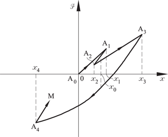
Copyright information

© CIMNE, Barcelona, Spain 2017